What MyoVision did
Algorithm worflow
When you ran the example, MyoVision:
- opened a configuration file (
configuration_data.xml) stored in..\demos\example_A\configuration_data.- looked at the task file section
- saw one task specified with
- an input image file
PoWer_3_Gastroc_10x_blue_cropped_small.pngstored in..\demos\example_A\raw_image - results to be written to
..\demos\example_A\results
- an input image file
- saw one task specified with
- looked at the task file section
-
ran the task by:
-
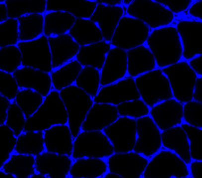
reading in the input image file
-
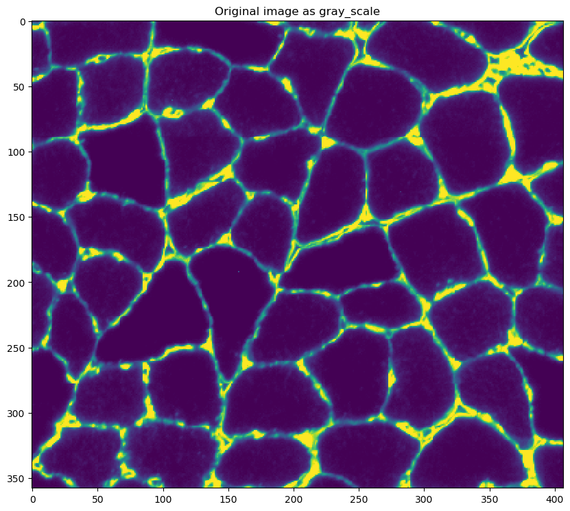
converting it to gray-scale
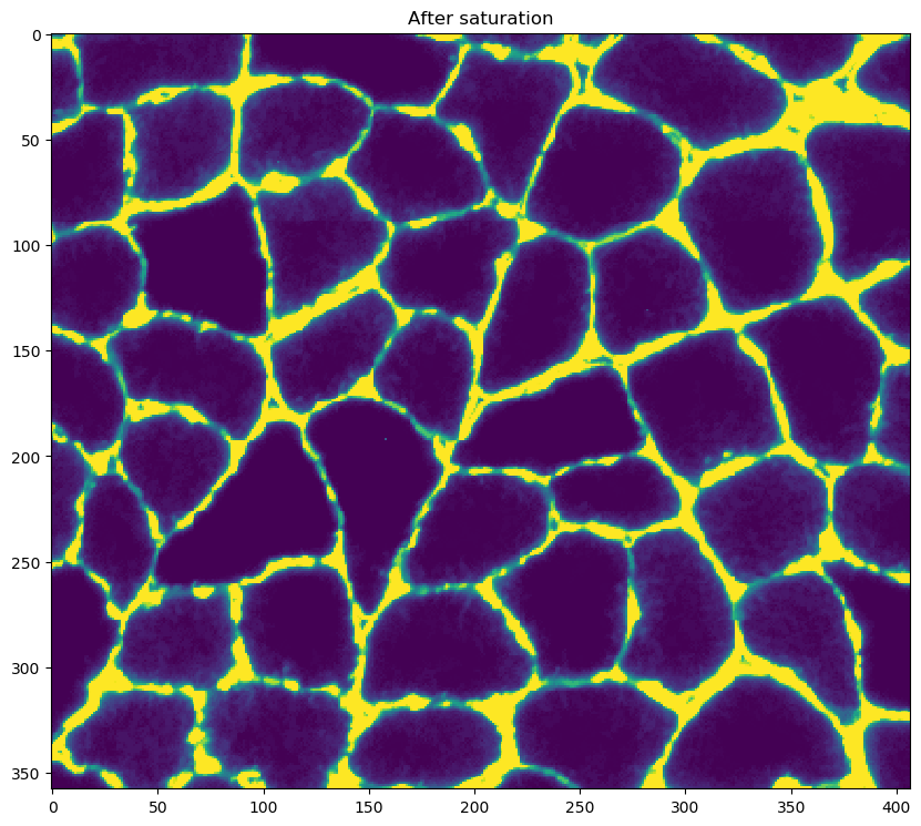
- saturating the image
- this step adjusts the brightness and contrast of the gray-scale image until x percent of the pixels are as dark as they can be, and x percent are as light as they can be
- the x value, in this case 10%, is set by the
saturation percentvariable in the<image_to_label_parameters>of the configuration file
-
enhancing the cell edges using a Frangi filter
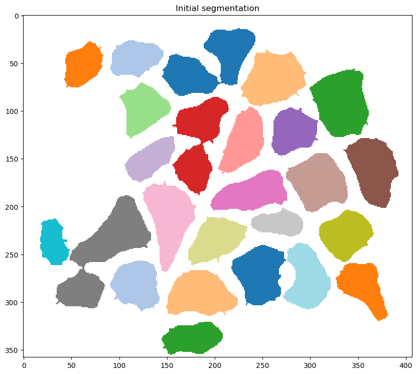
- performing an initial segmentation to identify ‘blobs’ - regions of connected pixels
- discarding blobs with an area below a critical size
- the critical size, in this case 50 pixels, is set by the
min_object_sizein the<image_to_label_parameters>of the configuration file
- loading a classifier model (more on this later) set by
classification_model_file_stringin the<classifier_parameters>section of the configuration file - using the classifier to mark each blob as one of the following:
- fiber
- potentially-connected fibers (two or more fibers separated by an incomplete cell boundary)
- something else
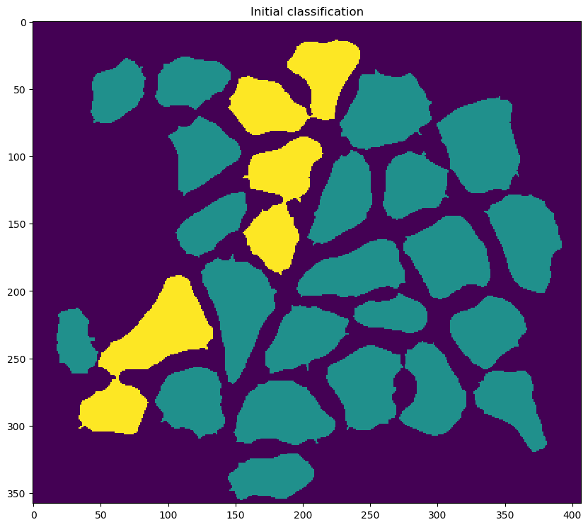
- attempting to separate potentially-connected fibers into single fibers
- this is done using a watershed algorithm and a
watershed_distance_parameter(in this case, 10 pixels) defined in the<image_to_label_parameters>section of the configuration file
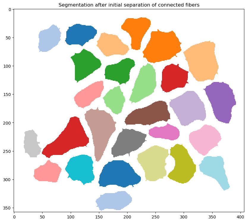
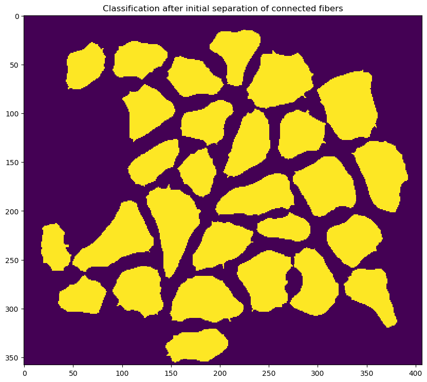
- this is done using a watershed algorithm and a
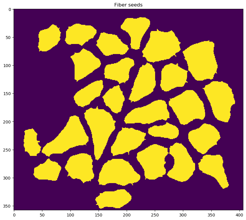
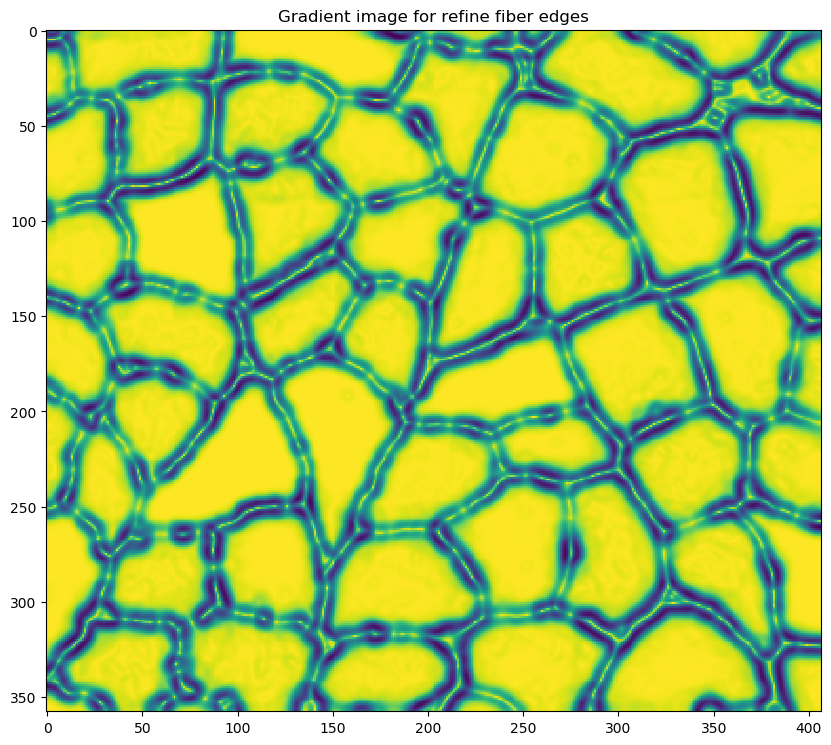
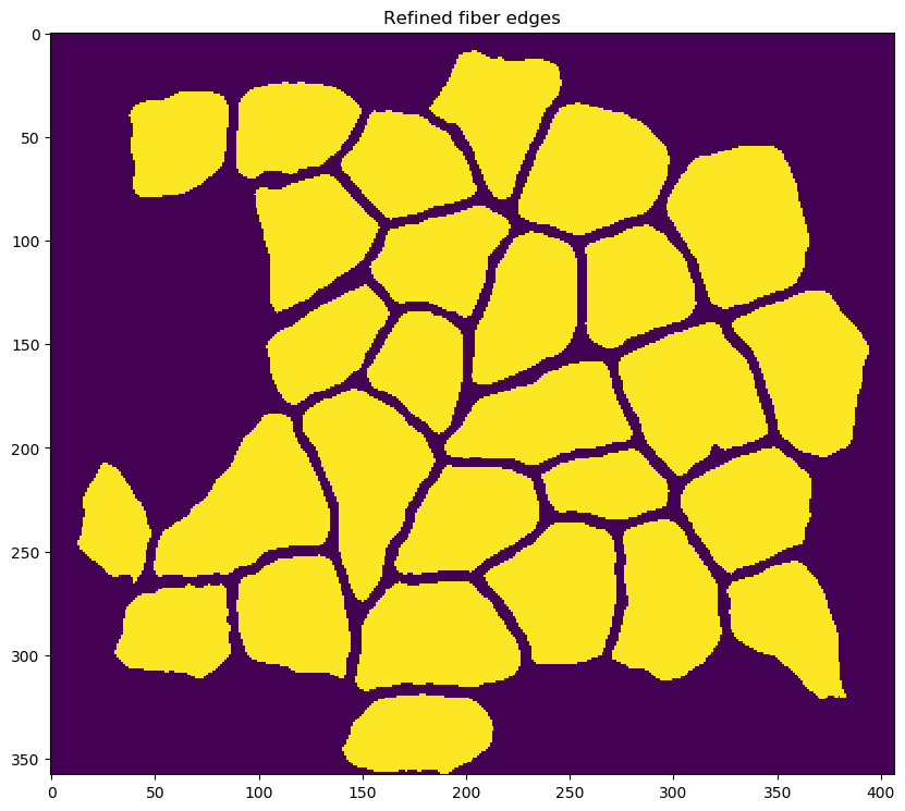
- refining the edges of each cell using an adaptive contour technique which depends on the following parameters which are defined in the
<refine_fibers_parameters>section of the configuration file:- max_iterations
- sigma
-
re-segmenting the image to identify fibers with improved fidelity


-
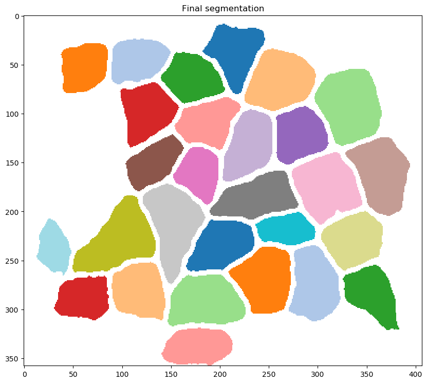
correcting for fibers that were inappropriately connected during the fiber refinement step

-
creating the following output files in
results_folder(which was specified for the task in the<task_files>section of the configuration file-
an Excel file
final_results.xlsxcontaining the following metrics for each fiber:- label (the id for the fiber)
- area (in pixels)
- eccentricity (0 is a circle, 1 is a straight line)
- convex area (in pixels)
- equivalent diameter (in pixels)
- extent (ratio of pixels in the blob to the pixels in the total bounding box)
- major axis length (in pixels)
- minor axis length (in pixels)
- orientation (angle between horizontal and the major axis of the equivalent ellipse - ranges from -pi/2 to +pi/2)
- perimeter (in pixels)
- solidity (ratio of pixels in the blob to the pixels in the convex hull image)
-
an image file
clean_overlay.pngshowing falsely-colored fibers overlaid on the original input image -
an image file
annotated_overlay.pngshowing falsely-colored fibers overlaid on the original input image with text labels showing the fiber IDs -
a zip file
processing.zipwhich can be useful for trouble-shooting and which contains:- a folder named
blockswith images showing processing steps for individual blocks - a folder named
classification_stepswith images showing the results of the processing steps outlined above
- a folder named
-
-