Start new analysis

This page provides simple instructions on performing a new analysis with GelBox.

Instructions

Using the GelBox through MATLAB:
- Launch MATLAB and navigate to the Apps tab on the top menu. Find the GelBox under My Apps and start the application by clicking it. The instructions on how to locate the Apps tab can be found here
Using the GelBox as a stand-alone application:
- Locate your GelBox.exe shortcut and start the application by double-clicking it.

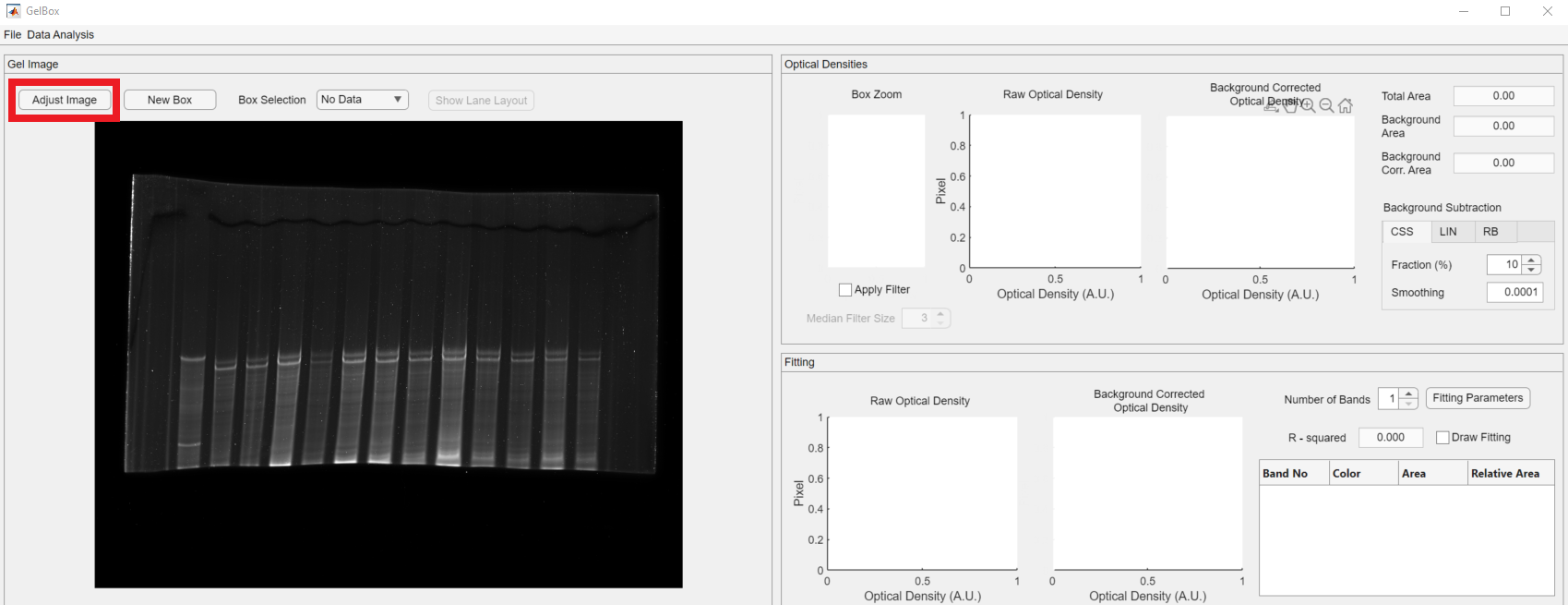
After a few seconds, you should see a program window. Here is the GelBox interface. (Clicking on any of the images on this page will open a larger version in a new browser window.).

The interface is divided into three different panels. Their functionality is summarized as follows:

Gel Image: The image axes display the gel images. The main region of interest (ROI) box controls are above the axes. Users can create ROI boxes.
Optical Densities: It shows the ROI’s raw and background corrected densitometry profiles. Box Zoom axes show an enlarged version of the enclosed area for a closer review.
Fitting: It shows the results of the curve fitting process. The main fitting controls are in this panel.

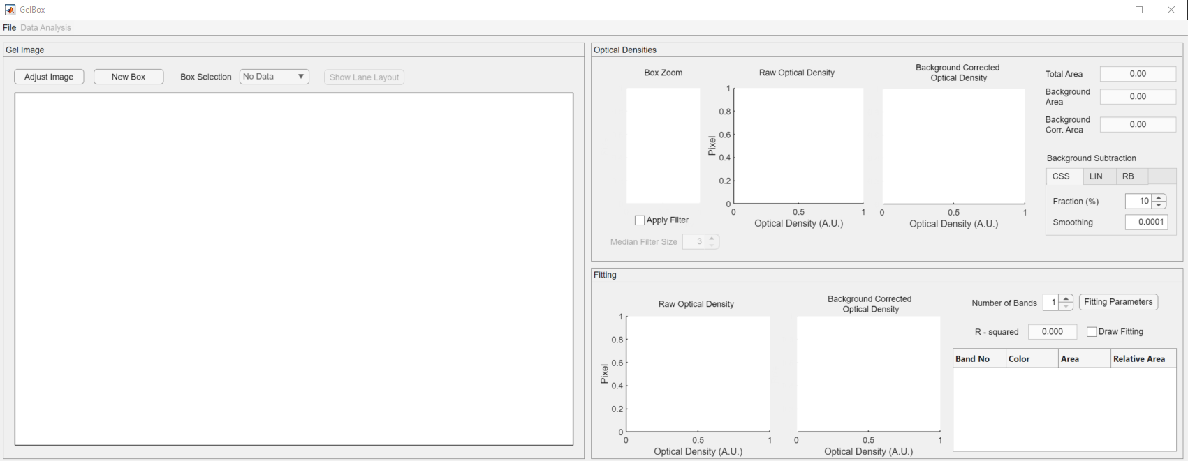
The first step of the analysis with GelBox is to load an image file to the environment. The File button on the top menu opens a dropdown menu, shown in a rectangle. The first option of the dropdown is the Load Image.

Upon clicking the Load Image button, it opens a normal Windows File Open Dialog. Locate the folder which has the gel images on your computer. GelBox can work with PNG (Portable Network Graphics), TIFF (Tag Image File Format), BMP (Bitmap), GIF (Graphics Interchange Formats), JPEG (Joint Photographic Expert Group), JPEG 2000, PBM (Portable Bitmaps), and PGM (Portable Gray Map) images. In this tutorial, the file format is selected as TIF in the red rectangle. This can be switched to PNG using the file extension dropdown. Select your gel image and click Open.

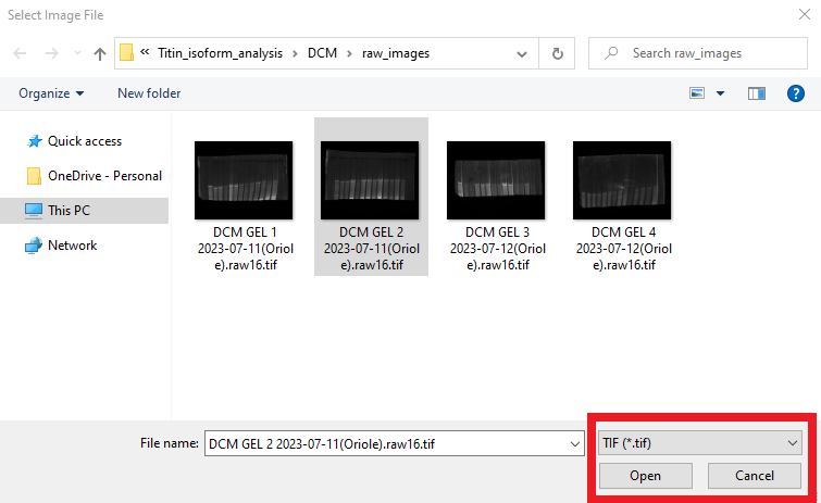
You can download the test image used in this tutorial here.

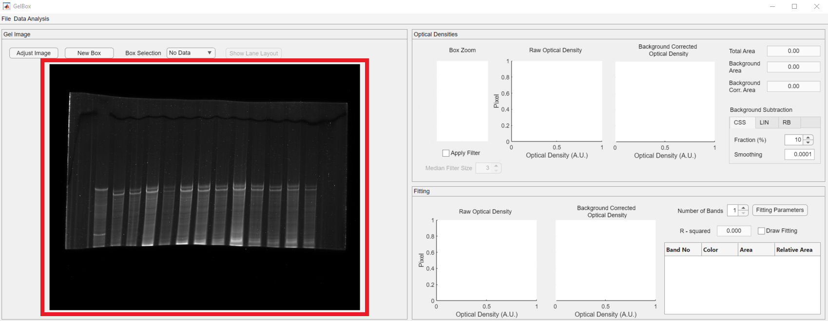
An image of your gel should now be displayed in the gel image panel (red rectangle).

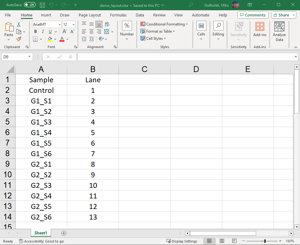
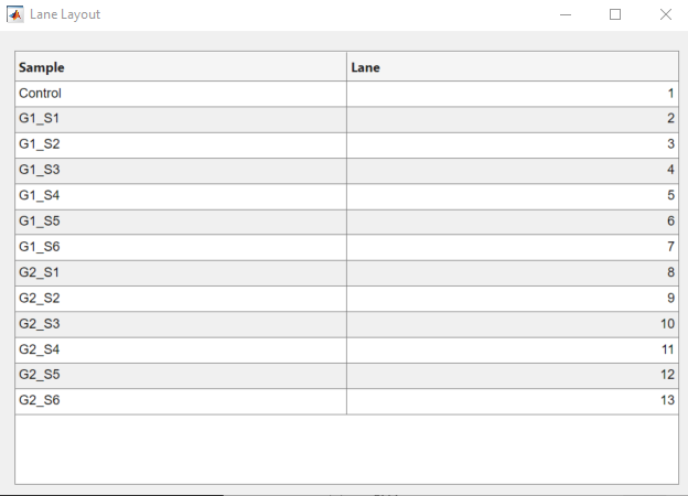
GelBox allows users to load their metadata consisting of information on the loaded samples. These data can be loaded in an Excel file. An example of metadata is given below. Following the analysis, the metadata will be combined with the analysis. GelBox requires the “Lane” column to be present in the layout file to perform this task.

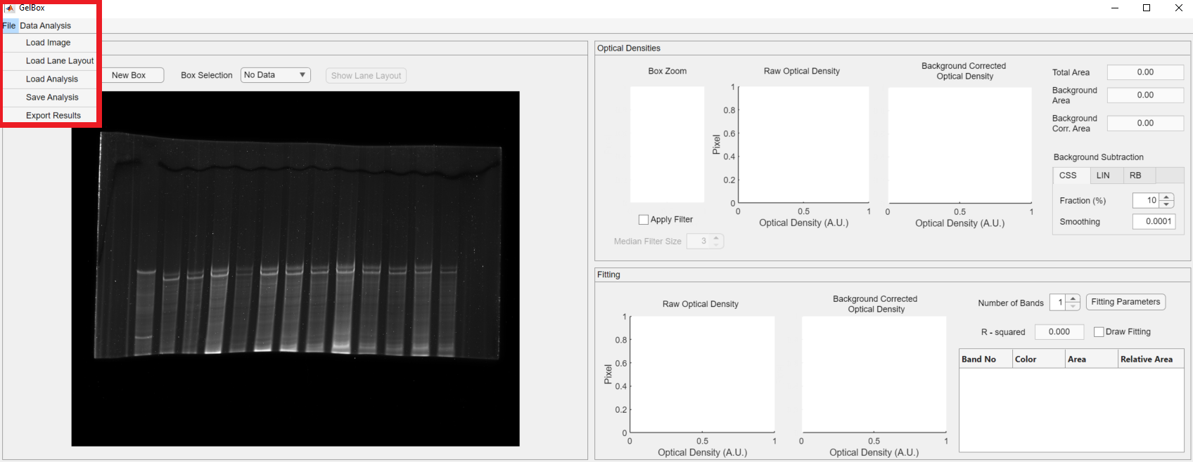
Click the file button on the top menu to access the options and click the Load Layout File button, shown in red rectangle.

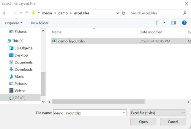
It opens a file dialog for you to locate the layout file.

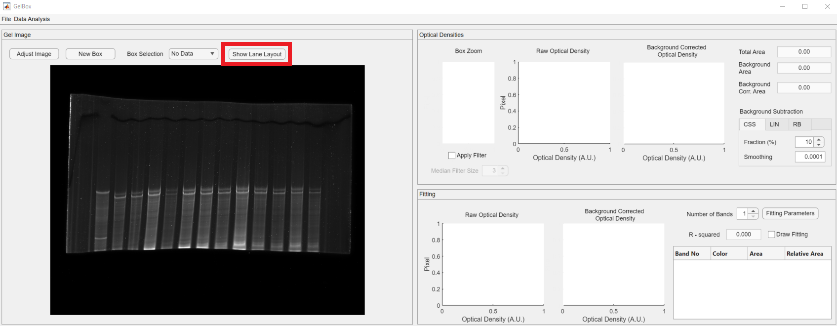
Upon loading the Excel file, you can review the layout using the Show Lane Layout button, shown in the red rectangle.

The layout table opens in a separate window.

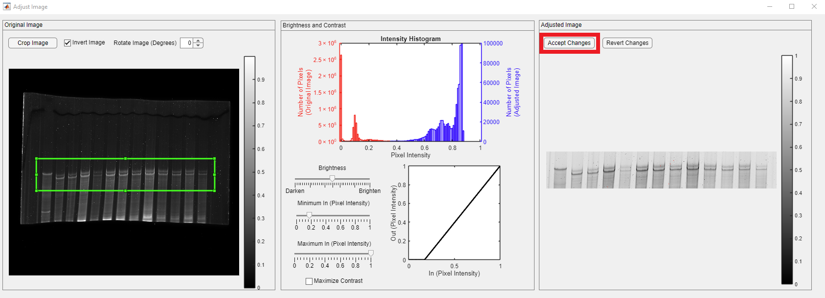
The loaded gel image has a darker background, and users can obtain a brighter background image using the GelBox’s built-in image adjustments window. To access the window, click the Adjust Image button in the red rectangle.

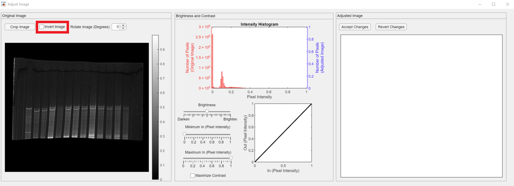
The Adjust Image has three main panels. Their functionality is summarized as follows:

Original Image: The loaded gel image before the modifications are shown in the panel. The color bar indicates the pixel intensity values in the image. The image adjustment controls are placed in the panel, namely Crop Image, Invert Image, Accept Changes, and Revert Changes.
Brightness and Contrast: It shows the pixel intensity histogram of the original (teal bars and left y-axis label) and the adjusted (purple bars and right y-axis label) image. The controls for brightness and contrast are placed in this panel.
Adjusted Image: It shows the adjusted image.

The Invert Image checkbox, shown in the red rectangle, lets users invert (darker pixels become brighter, and vice versa) their images.

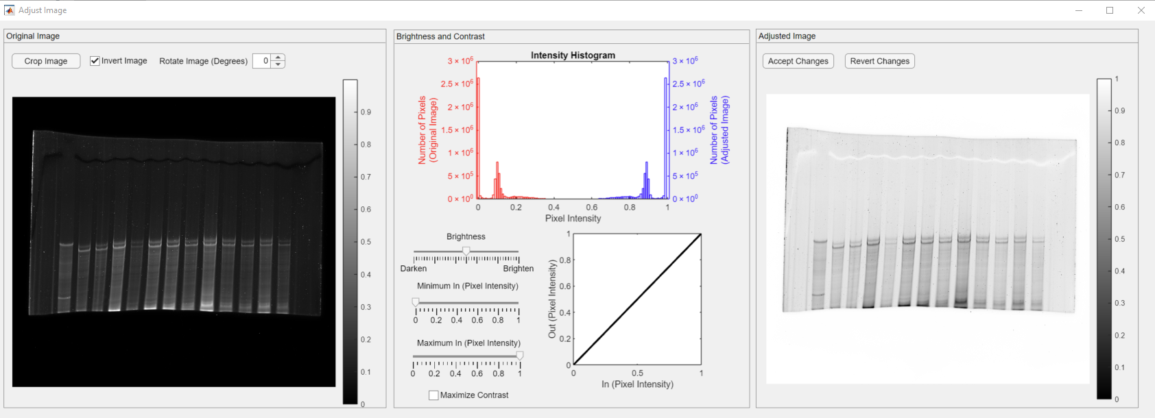
Upon clicking the Invert Image checkbox, the inverted image appears in the Adjusted Image panel.

Clicking the Invert Image button transforms bright pixels into dark pixels and vice versa. The inverted image appears in the Gel Image panel. In addition, the adjusted image intensity histogram appears in the plot. Please note that both red and blue histograms are symmetric.

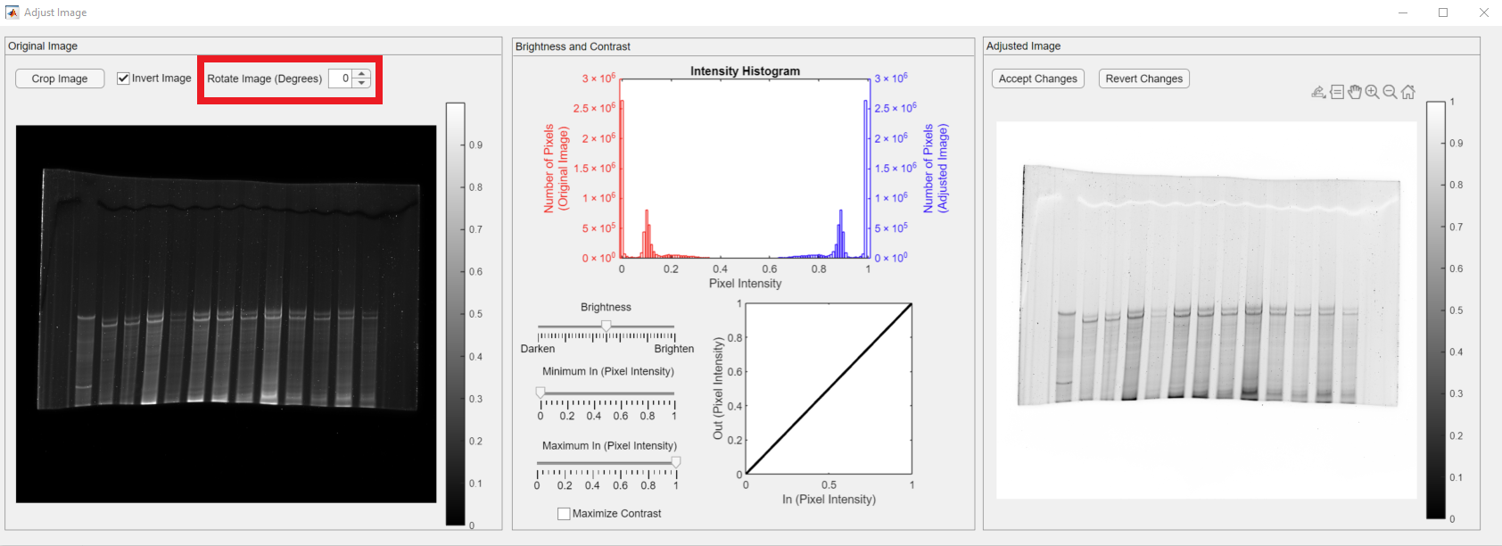
You can also rotate your image if needed using the Rotate Image spinner, shown in the red rectangle.

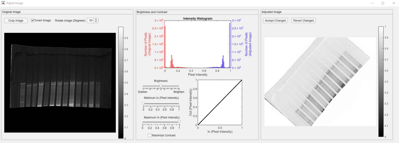
Set the angle to a desired value. the below example shows the image rotated by 50 degrees.

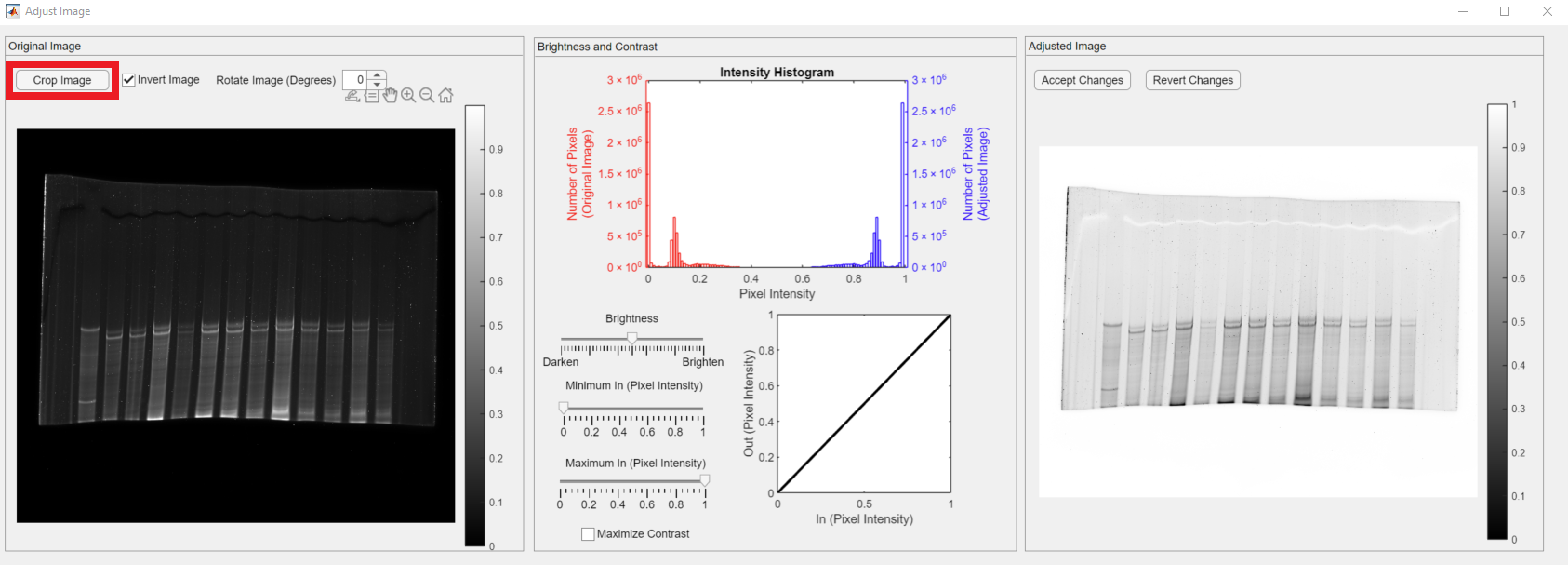
In this tutorial, the loaded gel image is a titin gel. We are interested in quantifying the relative quantities of cardiac N2B and N2BA titin isoforms. The first lane of the gel is loaded with a skeletal control sample. We are interested in the two bands that appeared around the mid-height of the gel. The rest of the gel image does not hold useful information. Therefore, the next step is to crop the image for the analysis. The Crop Image button, shown in the red rectangle, is in the Original Image panel.

The Crop Image button changes the mouse cursor into a crosshair and lets users select a rectangular enclosure (shown in green) in the original image. Please note that the adjusted image is changed to the cropped image and values on the right y-axis (purple) are reduced as the total number of pixels is decreased.

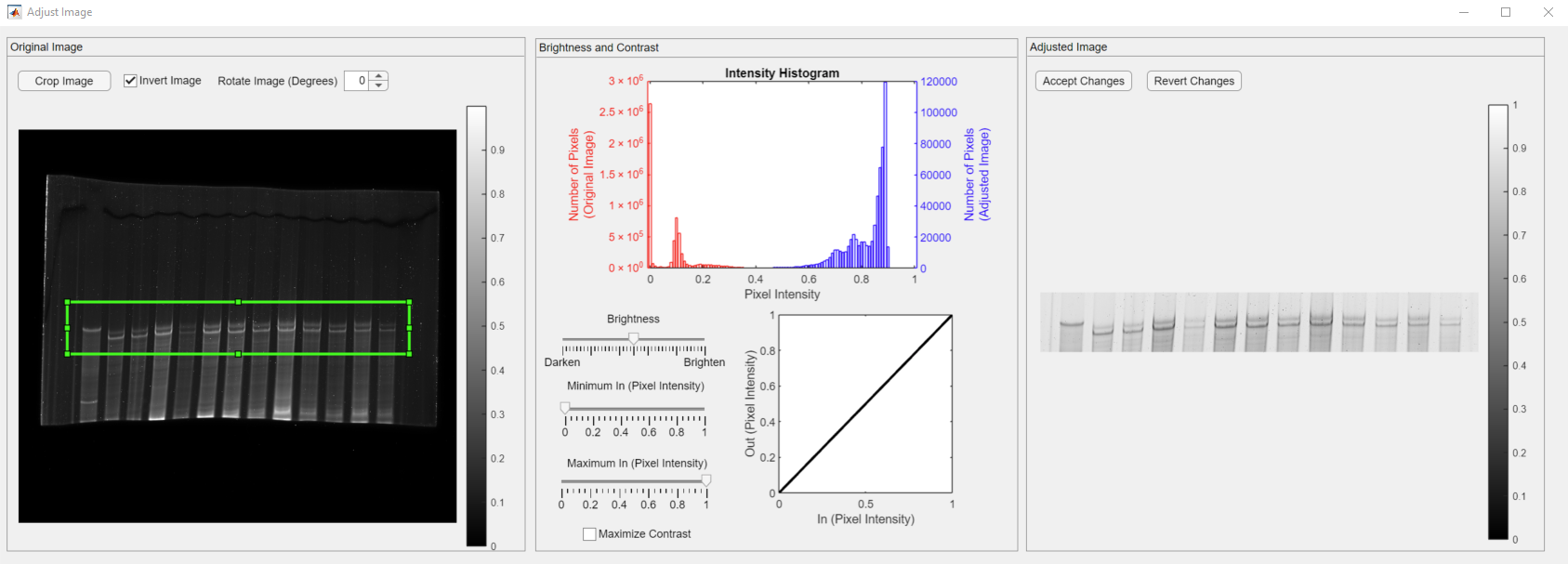
The box is stationary, yet it can be dragged around or resized. The histogram and the adjusted image displays would be updated in that case.

The visibility of the image can be adjusted by changing the brightness or adjusting the contrast by mapping the pixel intensities. During these operations, GelBox keeps track of the “over-saturated” pixels. If a pixel is “over-saturated,” it would be highlighted as red in the adjusted image panel. Please note that this feature is only for visual quality control purposes and will not modify the image with red pixels.

Once the image is adjusted and ready for quantification, click the Accept Changes button, shown in the red rectangle, to transfer the adjusted image to the GelBox environment.

Following the click the Adjust Image window is closed, and all the adjustments are stored for analysis export at the end.

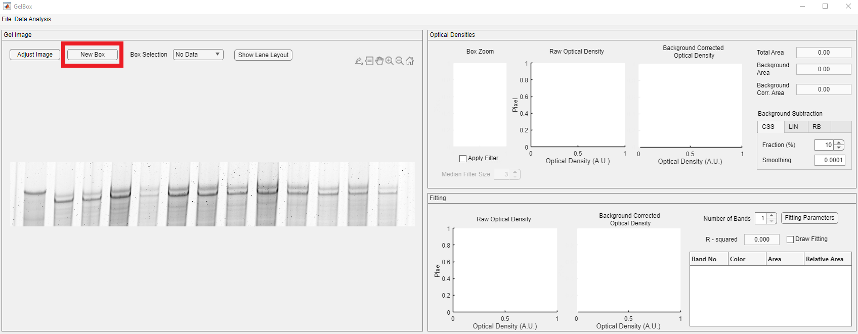
The next step is to draw an ROI box for analysis. Box controls are placed above the image axes, shown in red rectangle. After clicking the New Box button, the mouse cursor changes into a crosshair. Click on the image and expand the ROI to the desired size.

The newly generated box appears light green. The GelBox automatically processes the enclosed area in the ROI. Please note that all the empty axes and fields are populated now.

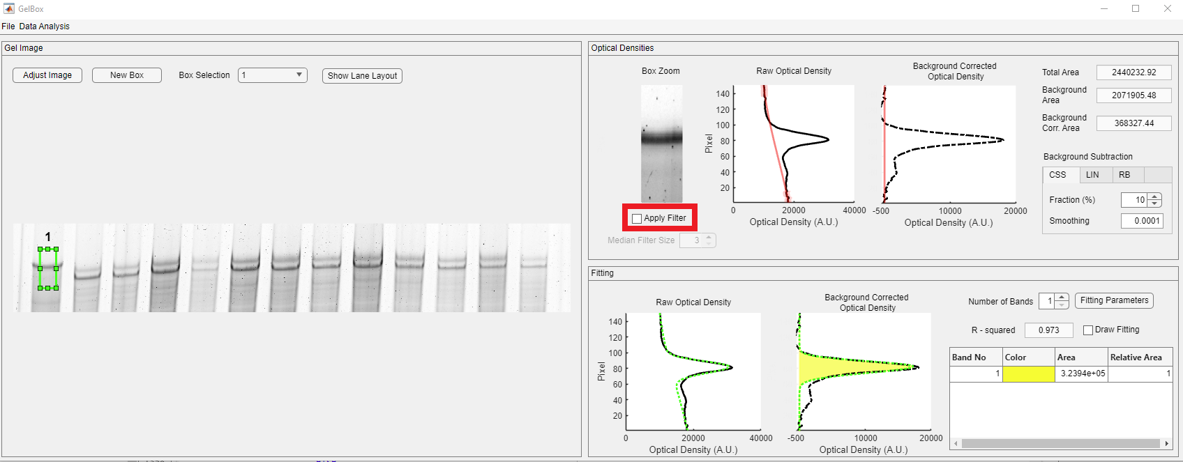
In the Optical Densities panel, the contents of the ROI are displayed in the Box Zoom axes. Please note that the Boz Zoom image can be seen to be darker than the original. It is because of MATLAB’s “scaled image display” option, in which the pixel intensities are scaled to the maximum available pixel intensity. This is used for display purposes and does not impact the calculation. The raw and background-corrected optical densities are shown in solid black and dashed black lines. The baseline is shown in the dashed magenta line. Background-corrected densitometry is obtained by subtracting the baseline from the raw density. Three different area values are automatically calculated.

- Total Area: The area under the raw densitometry profile
- Background Area: The area under the baseline
- Background Corr. Area: The area under the background corrected densitometry profile

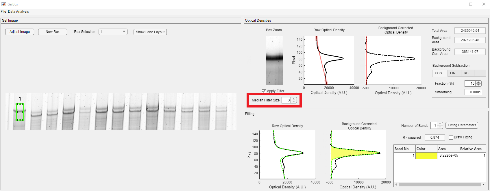
Users can apply median filtering to diminish the effects of the experimental artifacts, such as speckles. To apply median filtering to the ROI image, click the Apply Filter checkbox, shown in the red rectangle.

The default median filter size is 3, which defines the size of the square matrix around the center pixel. Users can change the filter size depending on the artifacts’ size. The Median Filter Size spinner is shown in the red rectangle below.

GelBox provides three different background correction methods to eliminate the effects of uneven background staining.

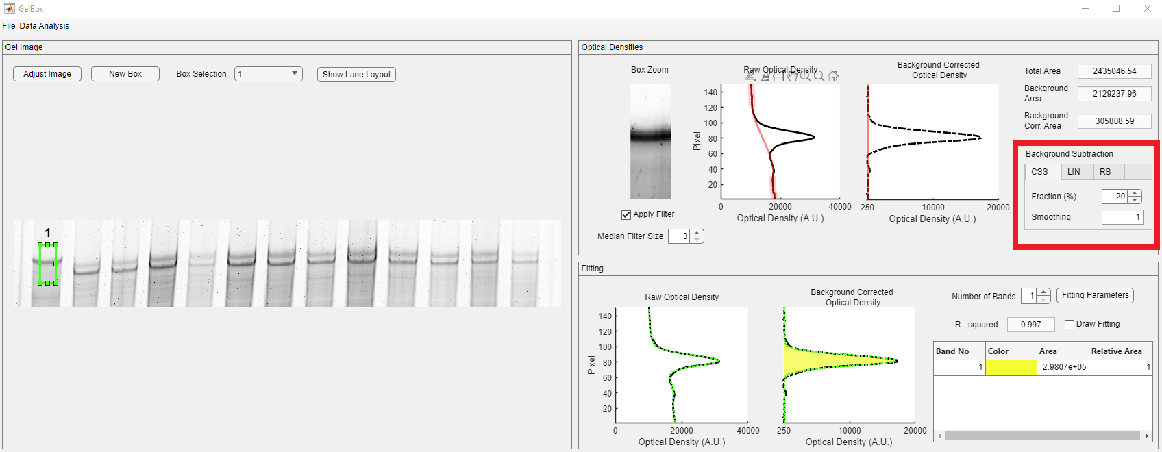
The cubic smoothing spline (CSS) method uses a fraction of the density profile from the top and the bottom of the density profile. The used points are highlighted in green circles on the Raw Optical Density plot. The default fraction is 10% and it can be adjusted using the Fraction spinner in the Background Subtraction tabbed display, shown in red rectangle. The smoothing parameter adjusts the roughness of the spline. The default option is 0.0001 and it can be adjusted using the Smoothing numeric edit field in the Background Subtraction tabbed display, shown in red rectangle.

As shown in the red rectangle below, the total number of points used in the CSS interpolation increased. This feature can be useful in noisy cases.

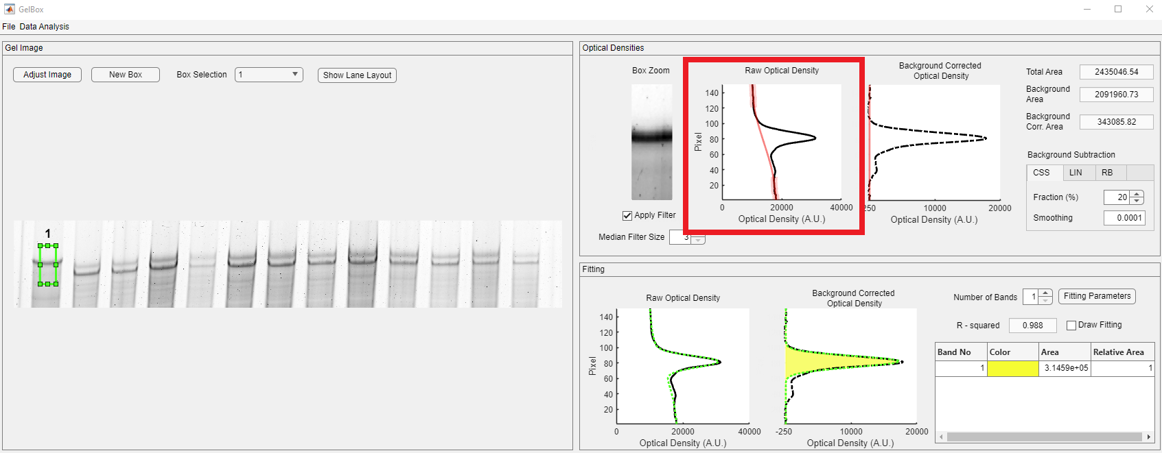
As shown in the red rectangle below, the curvature of the spline is changed.

The background correction method can be changed using the Background Subtraction tabbed display shown in the red rectangle.

The linear (LIN) method estimates the background by connecting the density profile’s beginning and end with a straight line.

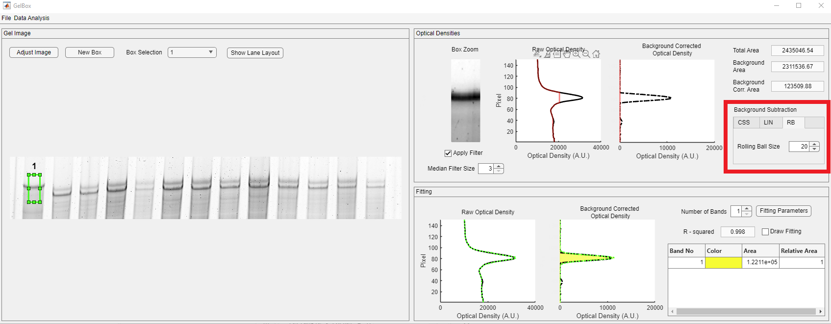
The third background correction option is the rolling ball (RB).

The rolling ball size should have a minimal impact on the quantification and converse as much raw data as possible. Users can change the rolling ball radius in pixels through the Rolling Ball Size spinner, shown in the red rectangle.

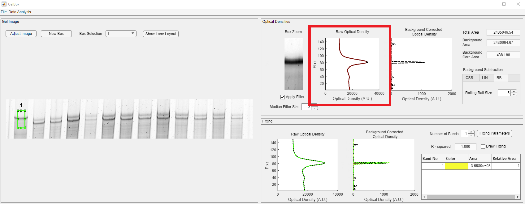
In the below example, the radius of 5 for the rolling ball removed almost all of the raw data, as highlighted in the red rectangle.

The tutorial continues with the CSS background correction method.

The box can be resized and moved along the image. The fitting process automatically follows the position of the box. You can explore a better fit by replacing or resizing the box.

Usually, there is more than one lane of interest in gels. Once you complete the current box, generate your next box as mentioned above. GelBox will automatically place a new box near the old box. All the boxes have the exact dimensions. The new box becomes the selected box (light green), and the old box is shown in red. Drag the new box to the desired position. Please note that the inset and density figures are updated as the box moves.

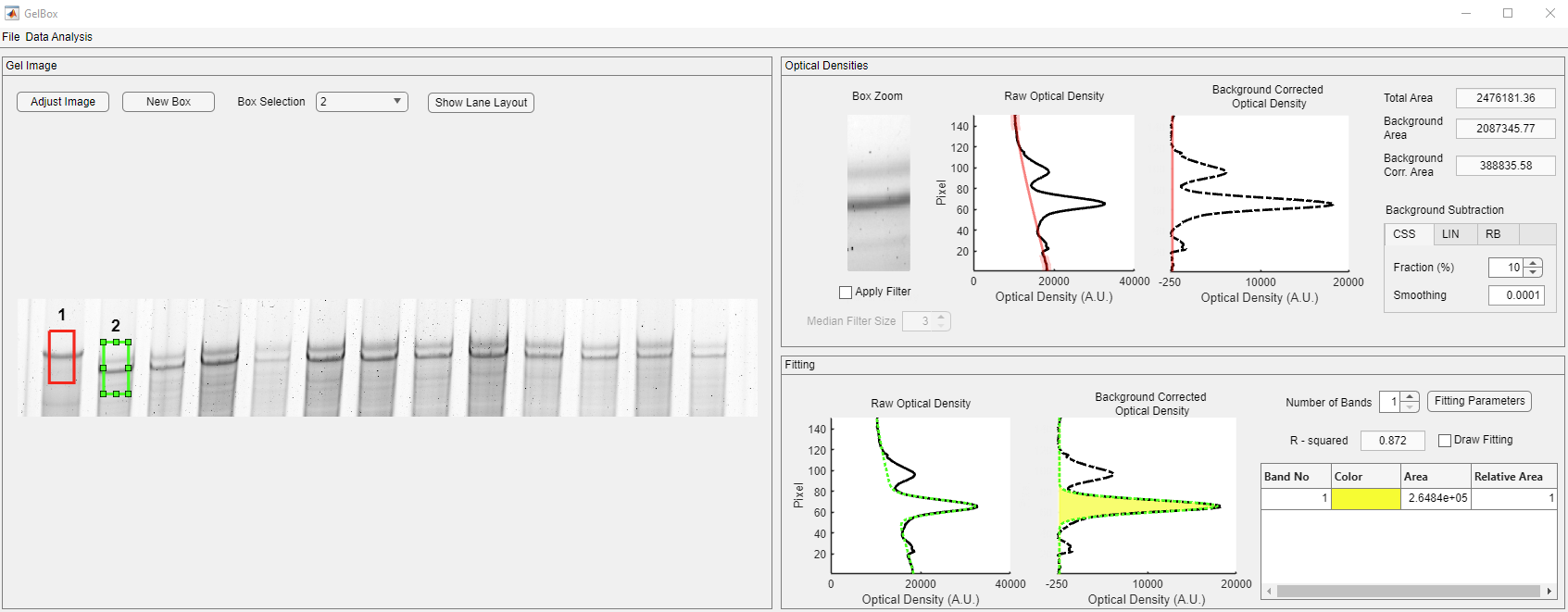
In the Fitting panel, the fitted function is displayed in a dashed green line in this panel. The yellow-shaded area in the Background Corrected Optical Density axes shows the area under the Gaussian function. The R-squared value is employed as a goodness-of-fit measure. The Band table shows the list of the bands and their color designation. The color designation follows the Parula colormap. The enumeration starts from the bottom of the density profile. The area is given in pixels, and the relative area is 1 as the number of bands is selected as one. Users can increase the number of bands in the ROI using the Number of Bands spinner, shown in the red rectangle. Upon changing the number of bands, GelBox automatically calculates the new Gaussian fit and updates all the fields. Please note that the color code has changed. While the purple-shaded area shows Band 1, the yellow-shaded area shows Band 2.

The relative quantities are calculated as:

Relative Quantities = Area of the Band of Interest / The Total Area of the Bands in the ROI.

Besides moving the box around the lanes, users can change the estimated fitting parameters to obtain better fits. The Fitting Parameters button in the red rectangle opens the fitting parameters table.

The window shows the tabulated estimated (beginning of the fitting) and calculated (end of the fitting) parameter values. The constraints are also listed in the table as checkboxes.

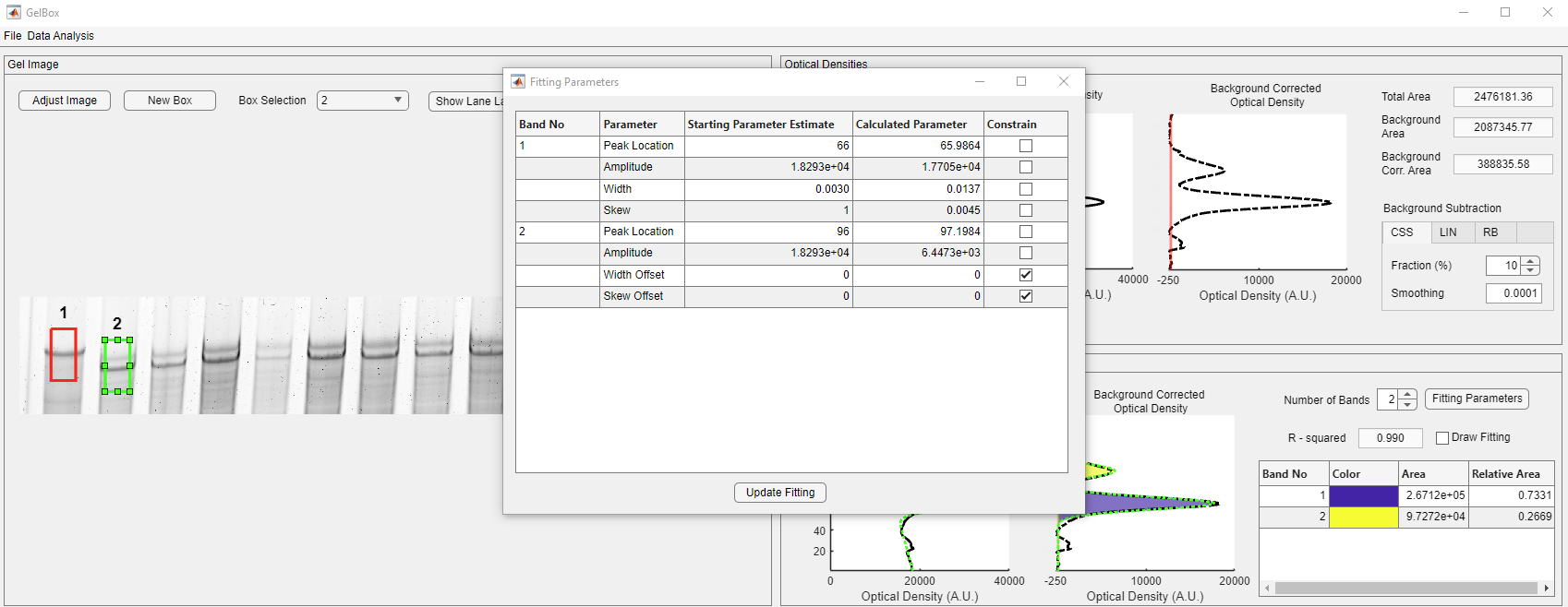
The width and the skew offset parameters are constrained to zero by default. Unchecking the highlighted box allows GelBox to adjust the widths of Gaussians separately. Once you uncheck the box, click the Update Fitting parameter button, shown in the red rectangle, to update the fits.

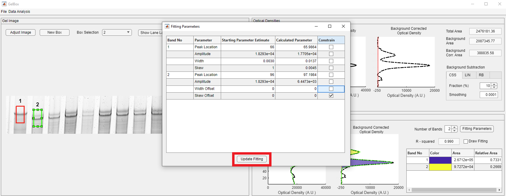
GelBox adjusts the parameters with the new constraint condition.

You can change the selected box using the Box Selection dropdown, shown in a rectangle.

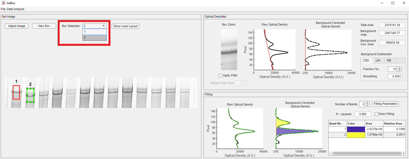
The second box can also be dragged around the image. However, when the selected box is resized, all the existing boxes also change size. Please note that the fits may change because of resizing. Make sure to check all the existing boxes to verify fits.

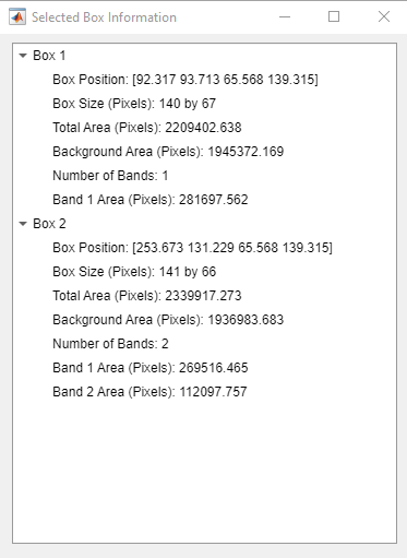
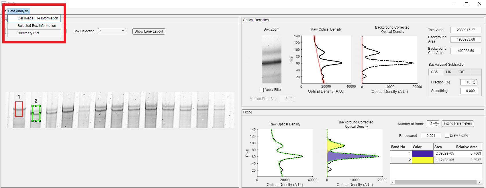
The new box positions, sizes, and area values can be accessed through the Selected Box Information window. Click the Data Analysis button on the toolbar in the red rectangle, then click the Selected Box Information.

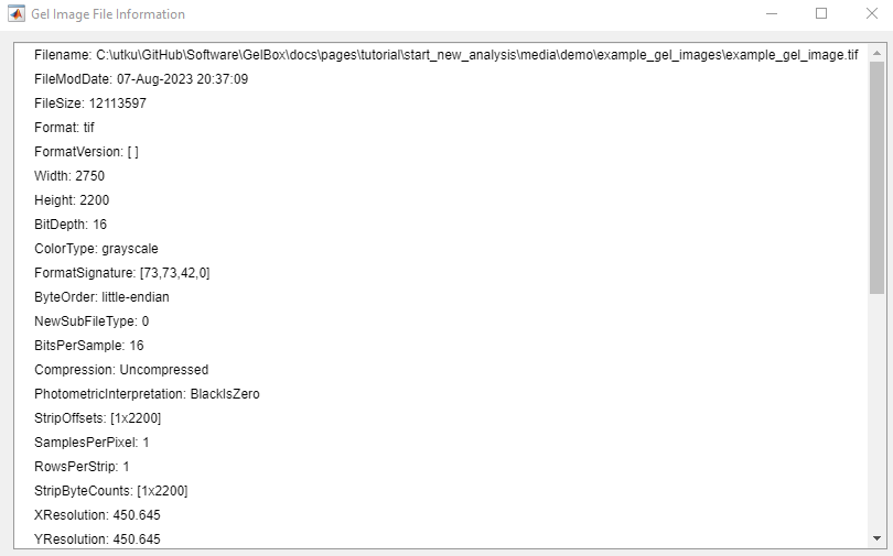
Users can also access the Gel Image Information window and review the stored image information. Click the Data Analysis button on the toolbar in the red rectangle, then click the Gel Image Information.

Here is the snapshot of the completed analysis.

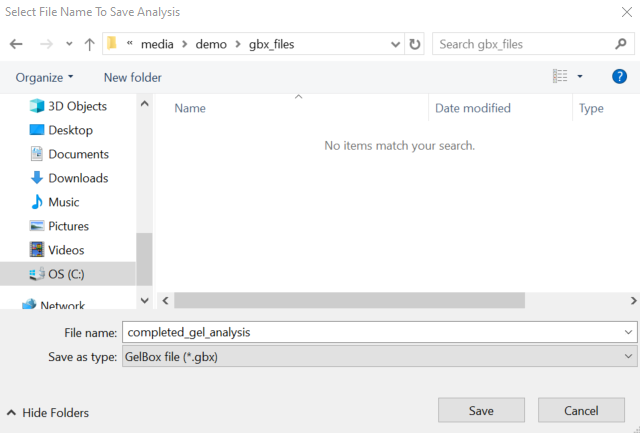
Once you finish your analysis, click the File button on the toolbar to save your analysis, shown in the red rectangle.

The Save Analysis button opens the following file dialog box, which allows you to save GelBox analysis files in a unique .gbx (short for GelBox) format. .gbx files store the raw image, adjusted image, analysis, and the used settings. This file format can be loaded to GelBox to revisit the analysis. Name your file and click Save.

In addition to the .gbx file, the settings are exported in a JSON (JavaScript Object Notation) file. The .gbx file and the settings JSON file take a little less than 12 MB of space, which makes them easy to share between researchers.

The settings JSON file has the following structure.

{
	"GelBox Settings": {
		"image_adjustments": {
			"crop_pos": [329.5579915,957.8658124,2126.878359,339.7353753],
			"brightness": 0,
			"contrast_lower": 0.1733333333,
			"contrast_upper": 1,
			"max_contrast": 0,
			"im_rotation": 0
		},
		"invert_status": 1,
		"filtering": {
			"median": {
				"size": [0,0,0,0,3,3,3,3,0,0,0,0,0]
			}
		},
		"background": {
			"method": [
				"Cubic Smoothing Spline (CSS)",
				"Cubic Smoothing Spline (CSS)",
				"Cubic Smoothing Spline (CSS)",
				"Cubic Smoothing Spline (CSS)",
				"Cubic Smoothing Spline (CSS)",
				"Cubic Smoothing Spline (CSS)",
				"Cubic Smoothing Spline (CSS)",
				"Cubic Smoothing Spline (CSS)",
				"Cubic Smoothing Spline (CSS)",
				"Cubic Smoothing Spline (CSS)",
				"Cubic Smoothing Spline (CSS)",
				"Cubic Smoothing Spline (CSS)",
				"Cubic Smoothing Spline (CSS)"
			],
			"css_fraction": [0.1,0.1,0.1,0.1,0.15,0.1,0.1,0.1,0.1,0.1,0.1,0.1,0.1],
			"css_smoothing": [0.0001,0.0001,0.0001,0.0001,0.1,0.001,0.001,0.001,0.001,0.001,0.001,0.001,0.001],
			"lin_fraction": [0,0,0,0,0,0,0,0,0,0,0,0,0],
			"rb_size": [0,0,0,0,0,0,0,0,0,0,0,0,0]
		}
	}
}

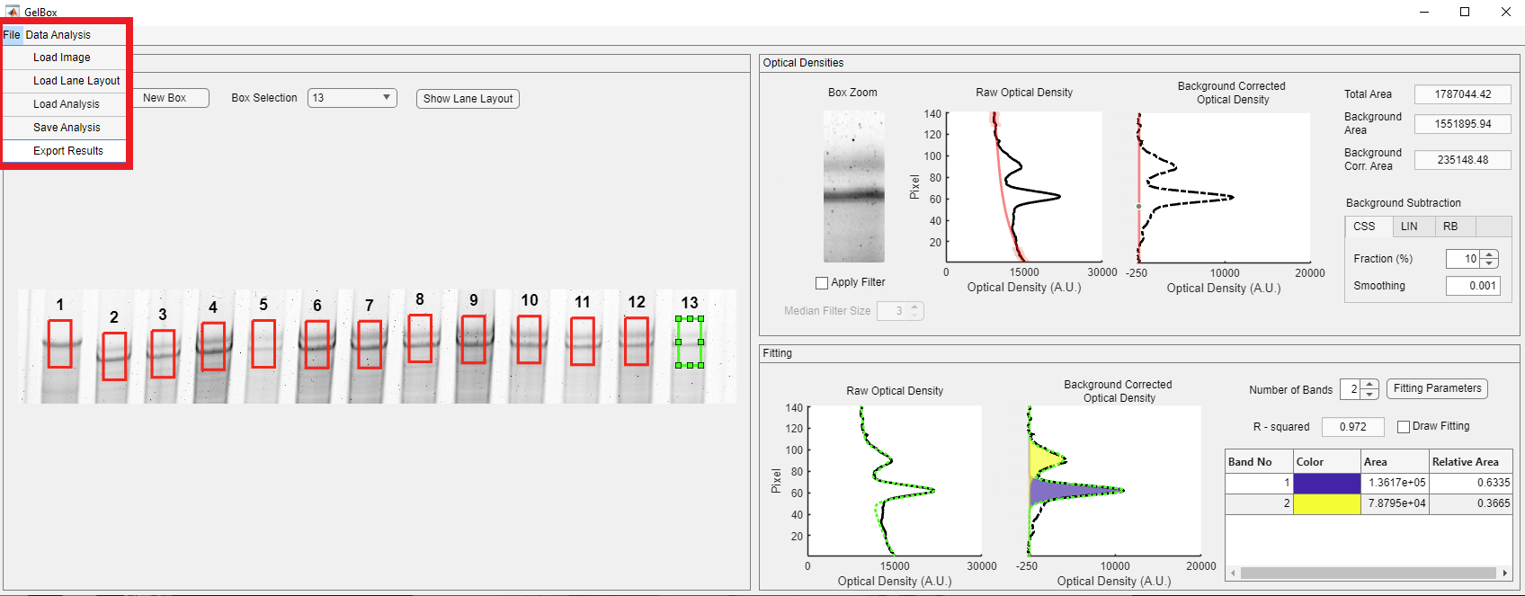
The Export Results button, shown in the red rectangle, opens a file dialog box for the analysis summary Excel file. You can combine your gel layout Excel files with the analysis Excel file to improve traceability.

First, GelBox asks users to select the name of the Analysis Results Excel file. Name your file and click Save.

Here is the snapshot of the Analysis Summary Excel file.

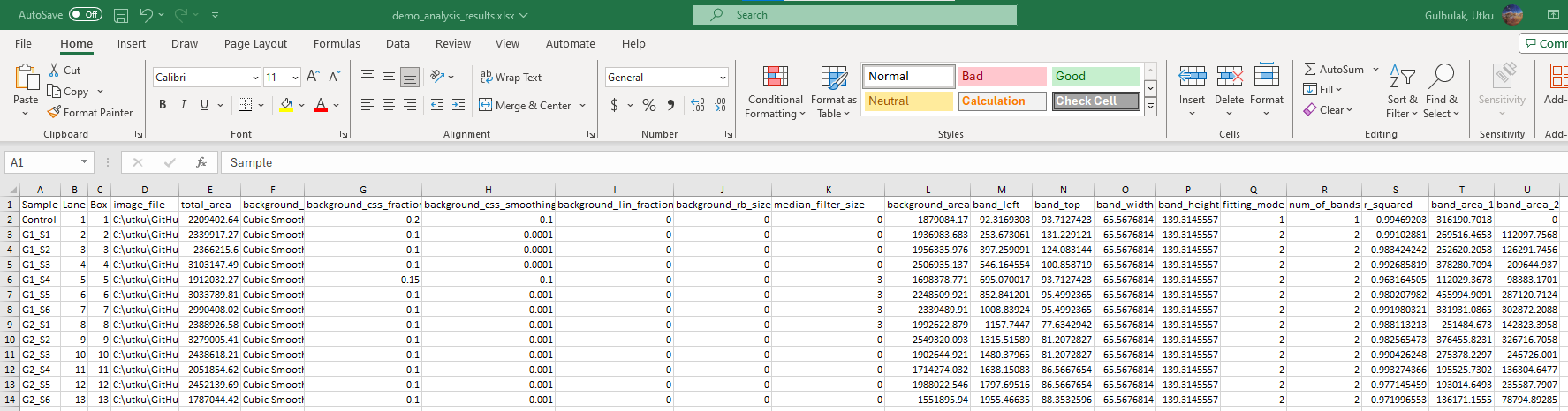
Summary Excel file has multiple sheets. The first sheet is the Summary sheet, and here are the brief descriptions of each column:

(Optional) Sample: Sample identifier
(Optional) Lane: The lane number in which the sample was loaded
Box: The box number
image_file: File path of the image
total_area: Area under the raw density trace
background_method: Implemented background correction method
background_css_fraction: The portion of the density profile used for cubic spline interpolation
background_css_smoothing: The smoothing parameter for the cubic spline
background_lin_fraction: The portion of the density profile used for linear interpolation
background_rb_size: The radius of the structural element
background_area: The Area under the baseline
band_left: Position of the upper left corner on the x-axis
band_top: Position of the upper left corner on the y-axis
band_width: Width of the box
band_height: Height of the box
fitting_mode: Number of Gaussian functions
num_of_bands: Number of bands
r_squared: R-squared value of the fit
band_area_1: Area under the first Gaussian function representing the first band
band_area_2: Area under the second Gaussian function representing the first band

The following sheets are named after the boxes. There is a sheet for each box in the analysis.

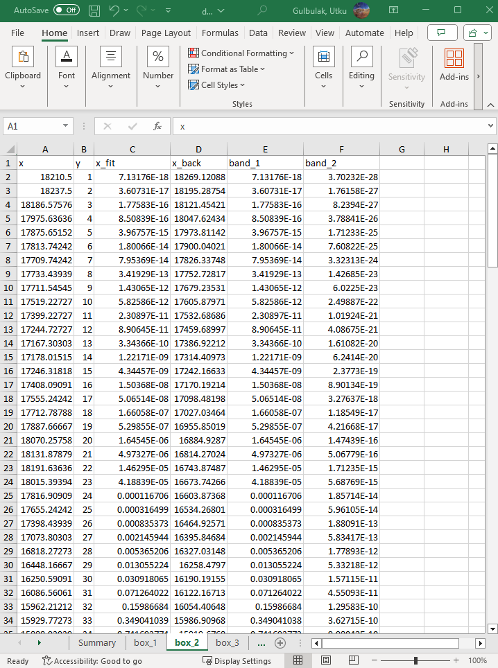
Here are the brief descriptions of each column.

x: Raw optical density value
y: Pixel index along the height of the box
x_fit: Fitted function value
x_back: Background density value
band_1: The first Gaussian function value
band_2: The second Gaussian function value

In addition, users can generate summary plots for their analysis. Click the Data Analysis button on the toolbar. The Summary Plot button is located at the bottom of the dropdown, shown in the red rectangle.

It opens the Summary Plot window. The window asks users to select the output folder, name the figure file, and define the band labels and the control lanes, if any.

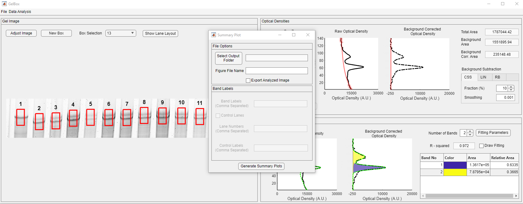
The Select Output Folder button opens the following folder dialog. Select your desired folder and fill in the rest of the fields. Then click the Generate Summary Plots button.

After a few seconds, the following figure appears and is saved under the selected folder.

The analyzed image is also exported. It can be found in the same folder as the summary plot.