Fitting pCa curves for two lengths
This demo shows how to fit simulations to two force pCa curves measured at different lengths assuming that the model parameters are the same for both curves.
The demo will be easier to follow if you have already looked at the fitting to a single pCa curve and fitting two condition pCa curves examples.
Instructions
- Launch MATLAB
- Change the MATLAB working directory to
<repo>/code/demos/fitting/two_length_tension_pCa - Open
demo_fit_two_length_tension_pCa.m - Press F5 to run the demo
Code
Here is the MATLAB code to perform the fit.
function demo_fit_two_length_tension_pCa
% Function demonstrates fitting a simple tension-pCa curve

% Variables
optimization_file_string = 'sim_input/optimization.json';

% Code

% Make sure the path allows us to find the right files
addpath(genpath('../../../../code'));

% Load optimization job
opt_json = loadjson(optimization_file_string);
opt_structure = opt_json.MyoSim_optimization;

% Start the optimization
fit_controller(opt_structure, ...
    'single_run', 0);
What the code does
The first 3 lines of (non-commented) code
- make sure the MATMyoSim project is available on the current path
- sets the file which definines an optimization structure
- loads the structure into memory
The last line of code calls fit_controller.m which runs the optimization defined in optimization.json
Optimization file
Here’s the optimization file. Predictably, it is very similar to the one described in fitting two condition pCa curves.
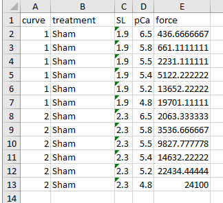
Again, the label in the curve column shows in the Excel file indicates which force values go with which curve in the target data.
{
	"MyoSim_optimization":
	{
        "model_template_file_string": "sim_input/model_template.json",

        "fit_mode": "fit_pCa_curve",
        "fit_variable": "muscle_force",

        "target_file_string": "target_data/target_force_pCa_data.xlsx",
        "target_field": "force",

        "best_model_folder": "temp/best",
        "best_opt_file_string": "temp/best/best_tension_pCa_model.json",

        "figure_current_fit": 2,
        "figure_optimization_progress": 3,

        "job":
        [
            {
                "model_file_string": "temp/1/65/model_worker_65.json",
                "protocol_file_string": "sim_input/1/65/protocol_65.txt",
                "options_file_string": "sim_input/sim_options.json",
                "results_file_string": "temp/1/65/65.myo"
            },
            {
                "model_file_string": "temp/1/58/model_worker_58.json",
                "protocol_file_string": "sim_input/1/58/protocol_58.txt",
                "options_file_string": "sim_input/sim_options.json",
                "results_file_string": "temp/1/58/58.myo"
            },
            {
                "model_file_string": "temp/1/55/model_worker_55.json",
                "protocol_file_string": "sim_input/1/55/protocol_55.txt",
                "options_file_string": "sim_input/sim_options.json",
                "results_file_string": "temp/1/55/55.myo"
            },
            {
                "model_file_string": "temp/1/54/model_worker_54.json",
                "protocol_file_string": "sim_input/1/54/protocol_54.txt",
                "options_file_string": "sim_input/sim_options.json",
                "results_file_string": "temp/1/54/54.myo"
            },
            {
                "model_file_string": "temp/1/52/model_worker_52.json",
                "protocol_file_string": "sim_input/1/52/protocol_52.txt",
                "options_file_string": "sim_input/sim_options.json",
                "results_file_string": "temp/1/52/52.myo"
            },
            {
                "model_file_string": "temp/1/48/model_worker_48.json",
                "protocol_file_string": "sim_input/1/48/protocol_48.txt",
                "options_file_string": "sim_input/sim_options.json",
                "results_file_string": "temp/1/48/48.myo"
            },
            {
                "model_file_string": "temp/2/65/model_worker_65.json",
                "protocol_file_string": "sim_input/2/65/protocol_65.txt",
                "options_file_string": "sim_input/sim_options.json",
                "results_file_string": "temp/2/65/65.myo"
            },
            {
                "model_file_string": "temp/2/58/model_worker_58.json",
                "protocol_file_string": "sim_input/2/58/protocol_58.txt",
                "options_file_string": "sim_input/sim_options.json",
                "results_file_string": "temp/2/58/58.myo"
            },
            {
                "model_file_string": "temp/2/55/model_worker_55.json",
                "protocol_file_string": "sim_input/2/55/protocol_55.txt",
                "options_file_string": "sim_input/sim_options.json",
                "results_file_string": "temp/2/55/55.myo"
            },
            {
                "model_file_string": "temp/2/54/model_worker_54.json",
                "protocol_file_string": "sim_input/2/54/protocol_54.txt",
                "options_file_string": "sim_input/sim_options.json",
                "results_file_string": "temp/2/54/54.myo"
            },
            {
                "model_file_string": "temp/2/52/model_worker_52.json",
                "protocol_file_string": "sim_input/2/52/protocol_52.txt",
                "options_file_string": "sim_input/sim_options.json",
                "results_file_string": "temp/2/52/52.myo"
            },
            {
                "model_file_string": "temp/2/48/model_worker_48.json",
                "protocol_file_string": "sim_input/2/48/protocol_48.txt",
                "options_file_string": "sim_input/sim_options.json",
                "results_file_string": "temp/2/48/48.myo"
            }
        ],
		"parameter": [
			{
				"name": "passive_hsl_slack",
				"min_value": 800,
				"max_value": 850,
				"p_value": 0.5,
				"p_mode": "lin"
			},
			{
				"name": "passive_k_linear",
				"min_value": 0,
				"max_value": 2,
				"p_value": 0.5,
				"p_mode": "log"
			},
			{
				"name": "k_1",
				"min_value": 0,
				"max_value": 1,
				"p_value": 0.5,
				"p_mode": "log"
			},
			{
				"name": "k_force",
				"min_value": -5,
				"max_value": -3,
				"p_value": 0.5,
				"p_mode": "log"
			},
			{
				"name": "k_3",
				"min_value": 0,
				"max_value": 2,
				"p_value": 0.50008379,
				"p_mode": "log"
			},
			{
				"name": "x_ps",
				"min_value": 0,
				"max_value": 5,
				"p_value": 0.5,
				"p_mode": "lin"
			},
			{
				"name": "k_on",
				"min_value": 7,
				"max_value": 8,
				"p_value": 0.4,
				"p_mode": "log"
			},
			{
				"name": "k_coop",
				"min_value": 0,
				"max_value": 1,
				"p_value": 0.3437755959,
				"p_mode": "log"
			}
		],
        "initial_delta_hsl": [0, 0, 0, 0, 0, 0, 200, 200, 200, 200, 200, 200]
    }
}
The only new feature in this file is the very last entry.
"initial_delta_hsl": [0, 0, 0, 0, 0, 0, 200, 200, 200, 200, 200, 200]
These values define an array of half-sarcomere lengths changes that are applied to the respective job at the very beginning of the simulation. Thus for jobs 7 through 12, the initial half-sarcomere length will be 950 nm (defined in the model_template_file plus 200 nm).
First iteration
As described for single pCa curve fit, the first iteration will produce 2 figures.
Fig 3 summarizes how the simulation matches the target data defined in the optimization structure.
- top panel, compares the current simulation to the target data
- middle panel, shows the relative errors for the different trials (although there is only 1 in this case)
- bottom panel, shows the parameter values
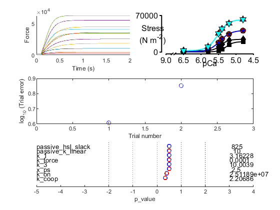
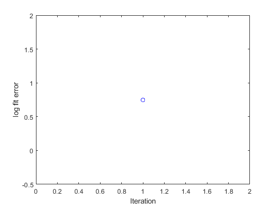
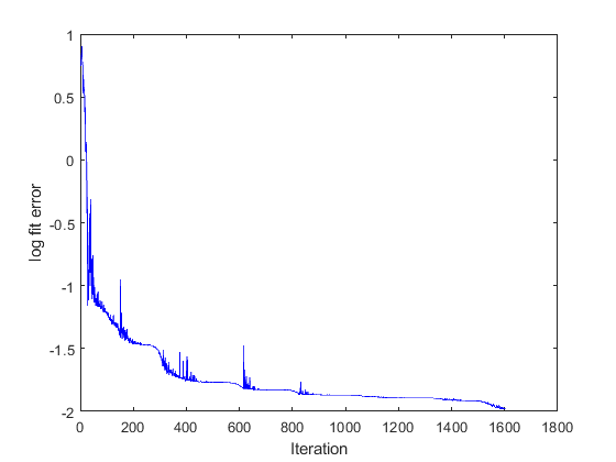
Fig 4 shows a single circle. This is the value of the error function which quantifies the difference between the current simulation and the target data. The goal of the fitting procedure is to lower this value in successive iterations.
Iterations
The code will continue to run simulations adjusting the values of the model parameters in successive iterations. As the calculations progress, the value of the error function will trend down, indicating that the fit is getting better.
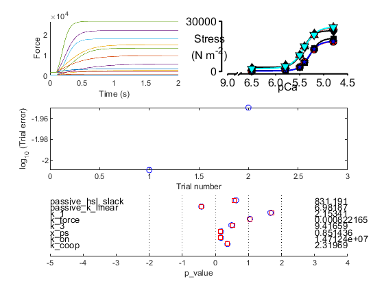
Final fit
The final summary and progress figures are shown below. Note that your progress figure might look slightly different because the optimization is based on randomly generated numbers.
Recovering the best fit
Each time the optimization process found a better fit, it
- updated the optimization template in
best_opt_file_string. This file is identical to the original optimization structure but with updated p values. - wrote the
model filesfor eachjobto thebest_model_folder.
You can recreate the best fitting simulation using these files. For example, you can update the demo code so that optimization file string points to temp/best/best_tension_pCa_model.json. If you also set the single_run option to 1 in the last line, the code will only create a single curve. That is, it won’t try and optimize a fit that should already be ‘optimal’.
If you need to access the data for individual simulations, you can load the *.myo files defined in the job structures. See other demos on how to do this.