Pendulum

Overview

This demo builds on the pendulum_1 demo and shows a pendulum connected to a muscle that is transiently activated.

What this demo does

This demo runs a single simulation with a pendulum

released from its zero position
connected to a MATMyoSim model that
- has passive stiffness
- is transiently activated by bursts of Ca²⁺

Instructions

In MATLAB, change the working directory to <repo>/code/demos/pendulum/pendulum_2
open demo_pendulum_2.m
Press F5 to run

Output

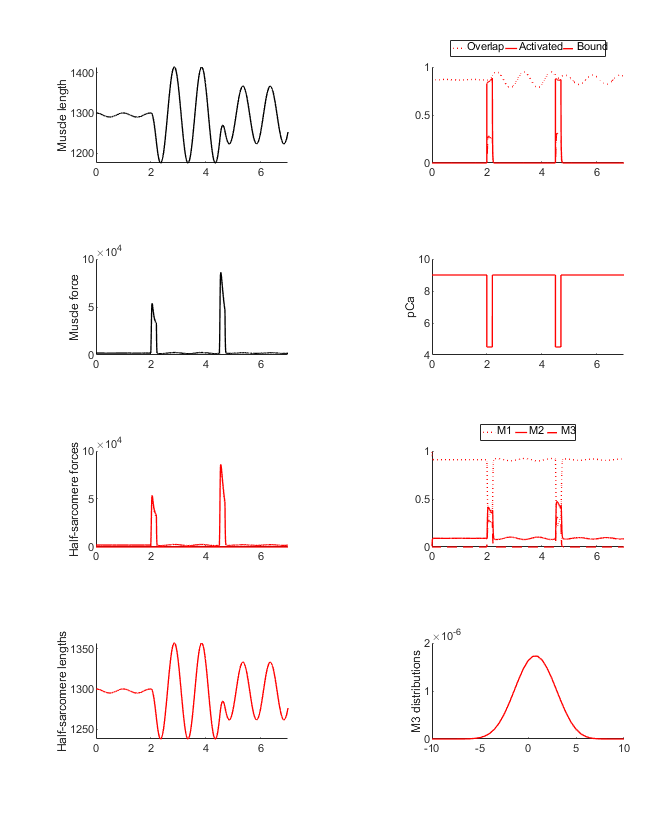
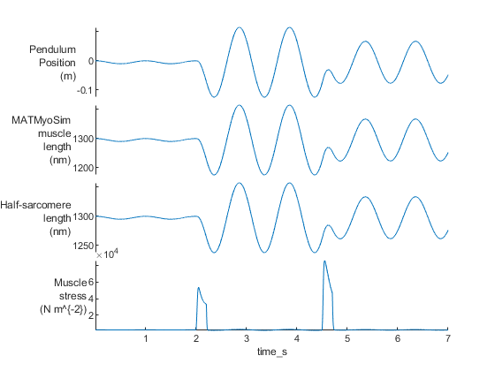
You should see two figures

and

How this worked

This demo is very similar to pendulum_1 demo except that the pendulum is started with an initial position of 0 and an initial velocity of 0. These are defined in the last entry in sim_input/pendulum.json.

{
    "pendulum":
    {
        "m": 10,
        "L": 0.25,
        "g": 9.81,
        "eta": 0,
        "hsl_scaling_factor": 500,
        "force_scaling_factor": 1e-3,
        "initial_conditions": [0.0, 0]
    }
}

The other key difference is that the MATMyoSim muscle is transiently activated by 2 bursts of Ca²⁺. These are defined in the demo_pendulum_2.m file.

% Brief activations
pCa(2000:2200) = 4.5;
pCa(4500:4700) = 4.5;

The first pulse generates a transient force that increases the magnitude of the pendulum’s swing. The second pulse is timed to partially brake the motion.

The first section of the demo code is

function demo_pendulum_1

% Variables
model_file = 'sim_input/model.json'
pendulum_file = 'sim_input/pendulum.json'
options_file = 'sim_input/options.json'
output_file = 'sim_output/output.myo'

% Make sure the path allows us to find the right files
addpath(genpath('../../../../code'));

% Create a simulation
sim = simulation(model_file)

% Set up a mini protocol with the number of time-points
% and pCa held at 9
no_of_time_points = 5000;
pCa = 9.0 * ones(no_of_time_points, 1);
dt = 0.001*ones(no_of_time_points,1);

This sets some filenames, updates the MATLAB path, and initialises a simulation based on a MATMyoSim model file.

The last three lines create a mini protocol with:

5000 time-points
each with a pCa value of 9.0
and a time-step of 0.001 s

The next section

% Implement the protocol
sim.implement_pendulum_protocol( ...
    'pendulum_file_string', pendulum_file, ...
    'options_file_string', options_file, ...
    'dt', dt, ...
    'pCa', pCa);

% Save the output
sim_output = sim.sim_output;

if (~isempty(output_file))
    % Check directory exists
    output_dir = fileparts(output_file);
    if (~isdir(output_dir))
        sprintf('Creating output directory: %s', fullfile(cd,output_dir))
        [status, msg, msgID] = mkdir(output_dir);
    end
    save(output_file,'sim_output');
end

implements the pendulum protocol and saves the output to a MATLAB file.

The last section

% Convert sim_output to a table - this requires deleting some fields
sim_output = sim.sim_output;
sim_output = rmfield(sim_output, 'myosim_muscle');
sim_output = rmfield(sim_output, 'subplots');
sim_output = rmfield(sim_output, 'no_of_time_points');
sim_output = rmfield(sim_output, 'cb_pops')
sim_output = struct2table(sim_output);

% Draw some of the output fields as a stacked plot
figure(3);
clf
stackedplot(sim_output, ...
    {'pendulum_position', 'muscle_length', 'hs_length', ...
    'hs_force'}, ...
    'XVariable', 'time_s', ...
    'DisplayLabels', { ...
        {'Pendulum','Position','(m)'}, ...
        {'MATMyoSim','muscle','length','(nm)'}, ...
        {'Half-sarcomere','length','(nm)'}, ...
        {'Muscle','stress','(N m^{-2})'}});

converts the output data to a MATLAB table and plots some of the key variables using the stackedplot function.

Interpretation

The sim_input/pendulum.json file defined the initial conditions of the pendulum as a position of 0.05 m and 0 velocity.

{
    "pendulum":
    {
        "m": 10,
        "L": 0.25,
        "g": 9.81,
        "eta": 0,
        "hsl_scaling_factor": 500,
        "force_scaling_factor": 1e-3,
        "initial_conditions": [0.05, 0]
    }
}

The activating Ca²⁺ concentration remained low throughout the simulation (pCa = 9.0 throughout) so the pendulum swung perturbed only by the passive stiffness of the MATMyoSim muscle.