Demo for tension-pCa

Overview

This demo shows how to

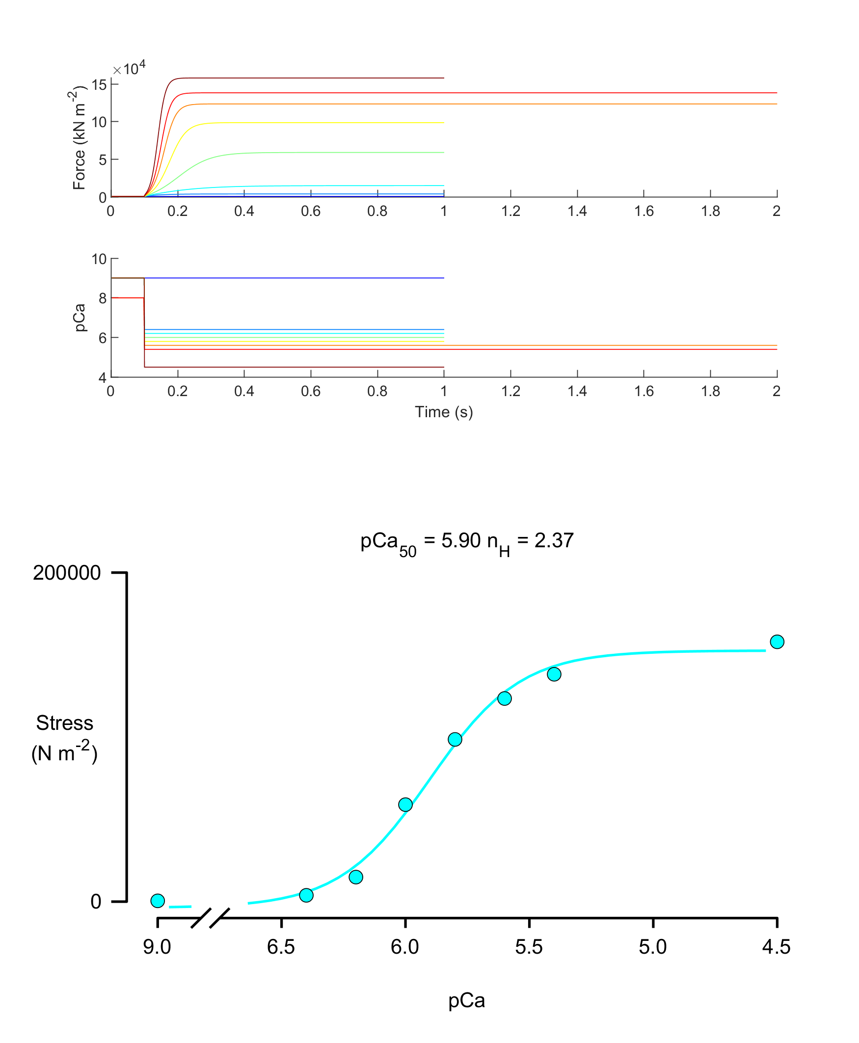
simulate isometric contractions at different levels of Ca²⁺ activation
fit a 4-parameter Hill-curve to the steady-state tension data

How this works

The demo initiates a set of simulations using a batch structure.

Each job in the batch defines a single simulation. A snippet of the file is shown here.

{
    "MyoSim_batch":
    {
        "job":
        [
            {
                "protocol_file_string": "sim_input/90/protocol_90.txt",
                "model_file_string": "sim_input/model_file.json",
                "options_file_string": "sim_input/sim_options.json",
                "results_file_string": "../../temp/sim_output/90/results_90.myo"
            },
            {
                "protocol_file_string": "sim_input/64/protocol_64.txt",
                "model_file_string": "sim_input/model_file.json",
                "options_file_string": "sim_input/sim_options.json",
                "results_file_string": "../../temp/sim_output/64/results_64.myo"
            },
            
            <SNIP>
        ]
    }
}

Note that every job uses the same

but a different

protocol

The results for each job are also written to different output files

Code

If you look at the demo code below, you can see that the function run_batch(batch_data) runs the entire set of simulations. (Behind the science, it uses a MATLAB parfor loop to run simulations on different threads in parallel.)

Once all of the jobs have finished, it is simple to extract the forces from each file and plot the resulting force-pCa curve.

function demo_tension_pCa
% Demo 

% Variables
batch_file_string = 'tension_pCa_batch.json';

% Make sure the path allows us to find the right files
addpath(genpath('../../../../code'));

% Load the batch data
batch_json = loadjson(batch_file_string);
batch_data = batch_json.MyoSim_batch;

% Run the batch
run_batch(batch_data);

% Make a figure showing each file and then plot pCa-force curve

% Make a figure
figure(1);
clf;
color_map = jet(numel(batch_data.job));

for i=1:numel(batch_data.job)
    
    % Load data
    sim = load(batch_data.job{i}.results_file_string, '-mat');
    sim_output = sim.sim_output;    
    
    % Plot force and pCa against time
    subplot(5, 1, 1);
    hold on;
    plot(sim_output.time_s, sim_output.muscle_force, '-', ...
        'Color', color_map(i,:));
    ylabel('Force (kN m^{-2})');
    
    subplot(5, 1, 2);
    hold on;
    pCa_trace = -log10(sim_output.Ca);
    plot(sim_output.time_s, pCa_trace, '-', ...
        'Color', color_map(i,:));
    ylabel('pCa');
    xlabel('Time (s)');
    
    % Keep force and pCa in a structure
    curve_data.pCa(i) = pCa_trace(end);
    curve_data.y(i) = sim_output.muscle_force(end);
    curve_data.y_error(i) = 0;
end

% Fit the tension-pCa curve
[curve_data.pCa50, curve_data.n_H, ...
    curve_data.passive_force, curve_data.active_force, ...
    curve_data.r_squared, curve_data.x_fit, curve_data.y_fit] = ...
        fit_Hill_curve(curve_data.pCa, curve_data.y);

% Plot
title_string = sprintf('pCa_{50} = %.2f n_H = %.2f', ...
                    curve_data.pCa50, curve_data.n_H);

plot_pCa_data_with_y_errors( curve_data, ...
    'axis_handle', subplot(2,1,2), ...
    'y_axis_label',{'Stress','(N m^{-2})'}, ...
    'y_label_offset', -0.1, ...
    'title', title_string);

If you want to extend this demo yourself, the folder also contains a function generate_protocols.m which creates activation protocols for a sequence of pCa values.

Instructions

Launch MATLAB
Change directory to the <repo>\code\demos\getting_started\tension_pCa folder in MATLAB
Open demo_tension_pCa.m
Press F5 to run the demo

Output

tension_pCa_output