Actin

Actin regulatory units are composed of binding sites that can transition from an inactive state to an active state, and vice-versa, as schematized below:

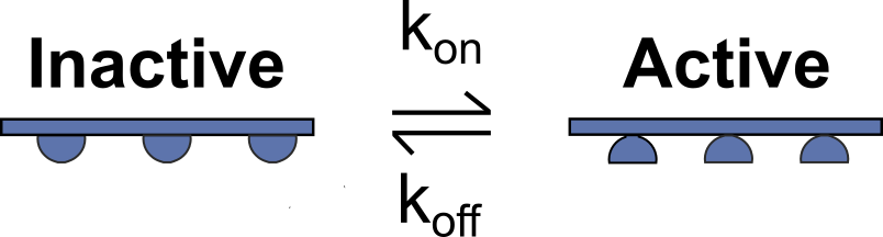
At each time step, all the binding sites from a regulatory unit can transition together according to the rate constants a_k_on and a_k_off defined in the model file. The probabilty of a regulatory unit activating is calculated using \(a_{k_{on}} [Ca^{2+}]\), and the probability of a regulatory unit deactivating is calculated using \(a_{k_{off}}\). These probabilities are also modulated by a_k_coop, which is a parameter quantifiying the inter-regulatory unit cooperativity:

• If no direct neighboring unit is activated, the activation rate is given by:

  \[a_{k_{on}} [Ca^{2+}]\]

• If one direct neighboring unit is already activated, the activation rate is given by:

  \[a_{k_{on}} [Ca^{2+}] (1 + a_{k_{coop}})\]

• If the two direct neighboring units are already activated, the activation rate is given by:

  \[a_{k_{on}} [Ca^{2+}] (1 + 2 \, a_{k_{coop}})\]

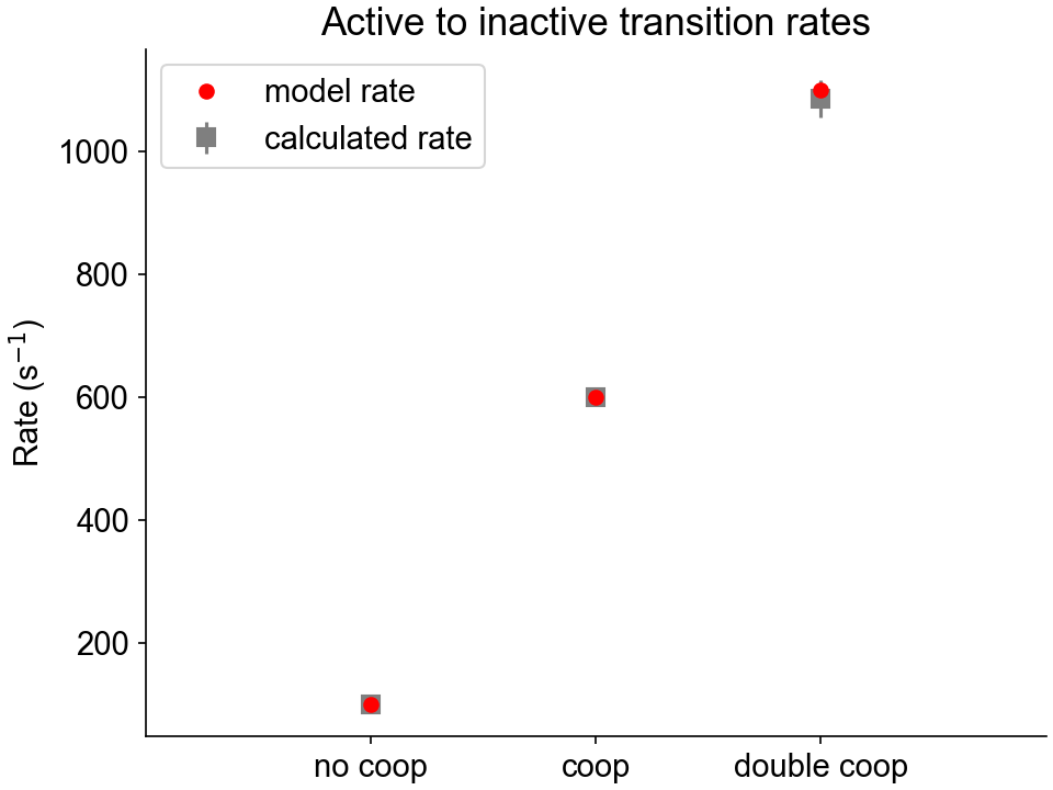
The same reasoning goes for the inactivating rate constant \(a_{k_{off}}\).

What this test does

The actin kinetics test:

• Runs a simulations in which a half-sarcomere is held isometric and activated in a solution with a pCa of 6.0.

• Saves a status file at each time step, which contains the state of every regulatory unit.

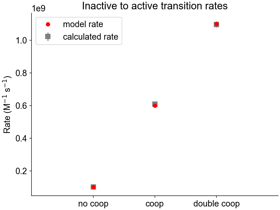
• Assesses all the regulatory units state transitions occuring between two consecutive time-steps, and calculates the apparent rate constants.

• Compares the calculated rate constants with those provided in the model file.

The batch file containing the instructions for this test is:

{
  "FiberSim_batch": {
    "FiberCpp_exe": {
      "relative_to": "this_file",
      "exe_file": "../../bin/FiberCpp.exe"
    },
    "job": [
      {
        "relative_to": "this_file",
        "model_file": "sim_input/model.json",
        "options_file": "sim_input/options.json",
        "protocol_file": "sim_input/pCa6_protocol.txt",
        "results_file": "sim_output/results.txt",
        "output_handler_file": "sim_input/output_handler.json"
      }
    ],
    "batch_validation": [
      {
        "validation_type": "a_kinetics",
        "relative_to": "this_file",
        "model_file": "sim_input/model.json",
        "options_file": "sim_input/options.json",
        "protocol_file": "sim_input/pCa6_protocol.txt",
        "output_data_folder": "sim_output/analysis"
      }
    ]
  }
}

As explained above, this batch file consists in a single job. The block called batch_validation provides the type of validation that must be run and the necessary files information.

Instructions

Before proceeding, make sure that you have followed the installation instructions and that you already tried to run the single trials demos.

Getting ready

• Open an Anaconda Prompt

• Activate the FiberSim Anaconda Environment by executing:

  conda activate fibersim
  

• Change directory to <FiberSim_dir>/code/FiberPy/FiberPy, where <FiberSim_dir> is the directory where you installed FiberSim.

Run the test

• Type:

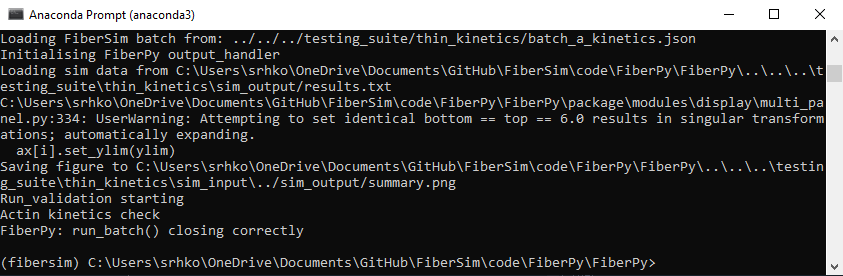
  python Fiberpy.py run_batch "../../../testing_suite/thin_kinetics/batch_a_kinetics.json"
  

• You should see text appearing in the terminal window, showing that the simulations are running. When it finishes (this can take ~15 minutes), you should see something similar to the image below.

Viewing the results

The results and summary figure from the simulation are written to files in <FiberSim_dir>/testing_suite/thin_kinetics/sim_output

The hs folder contains the status files that were dumped at each time-step calculation.

The analysis folder contains two figure files showing the calculated activating and deactivating rate constants for the three cooperative scenarios, as well as the model values.