Afterloads

Overview

This demo shows how to simulate twitches with afterloads.

What this demo does

This demo:

Runs a set of simulations in which a half-sarcomere is activated by a Ca²⁺ transient and allowed to shorten against a range of afterloads.

Instructions

If you need help with these step, check the installation instructions.

Open an Anaconda prompt
Activate the FiberSim environment
Change directory to <FiberSim_repo>/code/FiberPy/FiberPy

Run the command

 python FiberPy.py characterize "../../../demo_files/electrical_stimulation/afterloads/base/setup.json"

Viewing the results

All of the results from the simulation are written to files in <FiberSim_repo>/demo_files/electrical_stimulation/afterloads/sim_data/sim_output

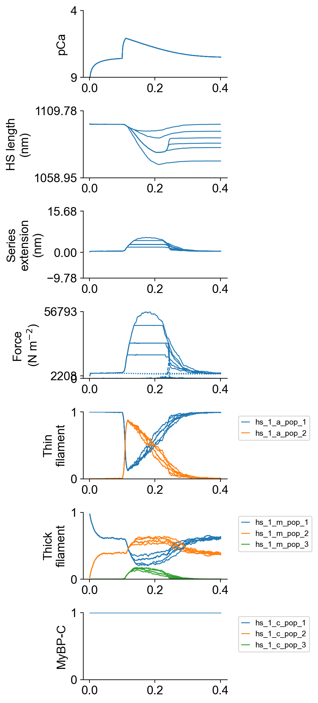
The file superposed_traces.png shows pCa, length, force per cross-sectional area (stress), and thick and thin filamnt properties plotted against time.

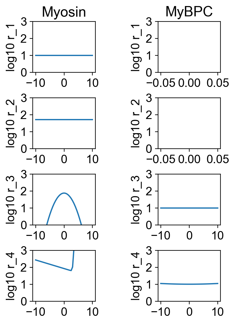
The file rates.png summarizes the kinetic scheme.

How this worked

The setup file is very similar to that used in the prior examples.

{
  "FiberSim_setup":
  {
    "FiberCpp_exe": {
      "relative_to": "this_file",
      "exe_file": "../../../../bin/FiberCpp.exe"
    },
    "model": {
      "relative_to": "this_file",
      "options_file": "sim_options.json",
      "model_files": ["model.json"]
    },
    "characterization": [
        {
            "type": "twitch",
            "relative_to": "this_file",
            "sim_folder": "../sim_data",
            "m_n": 9,
            "protocol":
            {
                "protocol_folder": "../protocols",
                "data": [
                    {
                        "time_step_s": 0.001,
                        "n_points": 400,
                        "stimulus_times_s": [0.1],
                        "Ca_content": 1e-3,
                        "stimulus_duration_s": 0.01,
                        "k_leak": 6e-4,
                        "k_act": 8.2e-2,
                        "k_serca": 20,
                        "afterload":
                        {
                            "load": [20000, 30000, 30000, 30000, 45000, 100000],
                            "break_delta_hs_length": [1, 1, 4, 8, 1, 1]
                        }
                    }
                ]
            },
            "output_image_formats": [ "png" ],
            "figures_only": "False",
            "trace_figures_on": "False"
        }
    ]
  }
}

The critical difference here lies in the characterization element.

The protocol->data element has a new component, labeled aferload.

 "afterload":
{
    "load": [20000, 30000, 30000, 30000, 45000, 100000],
    "break_delta_hs_length": [1, 1, 4, 8, 1, 1]
}

load and break_delta_hs_length are arrays (one value in each array for each simulation) defined as below.

Parameter	Sets
load	The muscle will remain isometric until the stress (N m^-2) equals this value, at which point the muscle will start to contract isotonically.
break_delta_hs_length	The maximum lengthening (in nm) allowed before the muscle breaks out of isotonic shortening and returns to isometric control at the prevailing length

Since there are 6 values in this example, the demo ran 6 separate trials.

Simulation	Comments
1	Afterload at 20000, break when lengthening exceeds 1 nm
2	Afterload at 30000, break when lengthening exceeds 1 nm
3	Afterload at 30000, break when lengthening exceeds 4 nm
4	Afterload at 30000, break when lengthening exceeds 8 nm
5	Afterload at 45000, break when lengthening exceeds 1 nm
6	Afterload at 100000, break when lengthening exceeds 1 nm. The muscle never generates this much force, so the entire simulation is isometric.