Parameter adjustments
Overview
This demo predicts how modulating the Ca2+ sensitivity of the thin filament and / or the rate of a myosin power stroke changes the force-pCa relationship and ktr.
What this demo does
This demo:
- Builds on the single pCa curve demo and runs simulations in which a half-sarcomere is subjected to a ktr maneuver at a range of pCa values
- Uses a
manipulationsstructure to create 4 models with different parameter values - Plots summaries of the simulation
Instructions
If you need help with these step, check the installation instructions.
- Open an Anaconda prompt
- Activate the FiberSim environment
- Change directory to
<FiberSim_repo>/code/FiberPy/FiberPy - Run the command
python FiberPy.py characterize "../../../demo_files/model_comparison/parameter_adjustments/base/setup.json"
Viewing the results
Notes Be aware:
- These simulations will look noisy because of the small
m_nvalue. - Even then, this code is running 36 simulations, so it may take ~10 minutes on a laptop.
All of the results from the simulation are written to files in <FiberSim_repo>/demo_files/model_comparison/parameter_adjustments/sim_data/sim_output
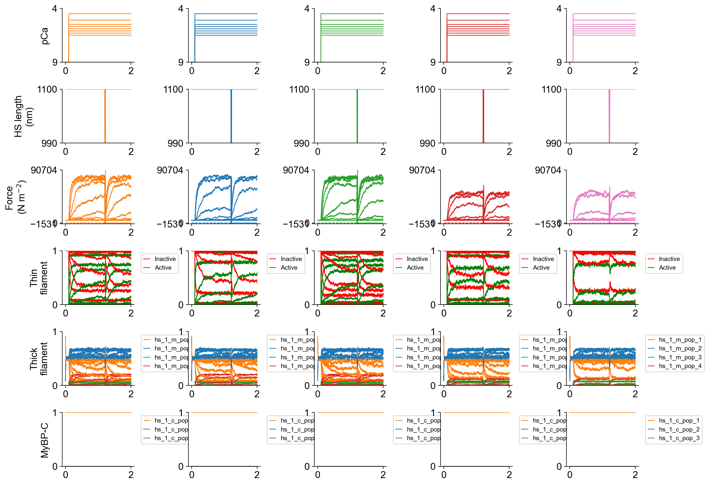
The file superposed_traces.png shows pCa, length, force per cross-sectional area (stress), and thick and thin filamnt properties plotted against time.
Since the simulations included more than 1 pCa value, FiberPy created a pCa curve force_pCa.png
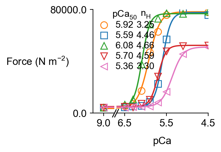
and wrote summary data to pCa_analysis.xlsx.
Since the code simulated a ktr maneuver, FiberPy also created a figure showing the analyis of the tension recovery.
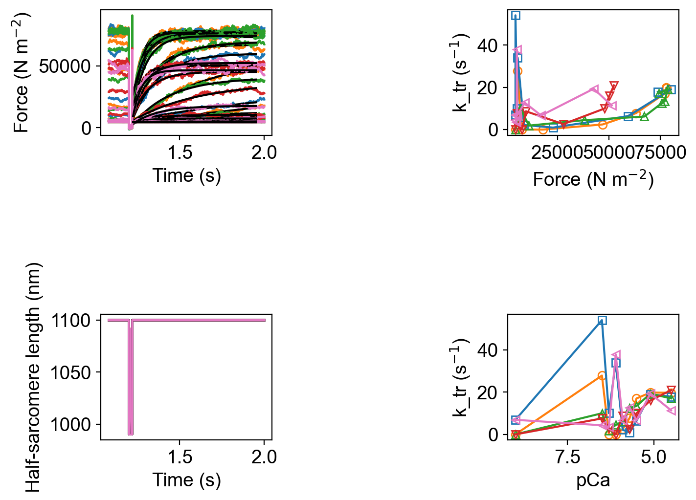
and wrote summary data to k_tr_analysis.xlsx.
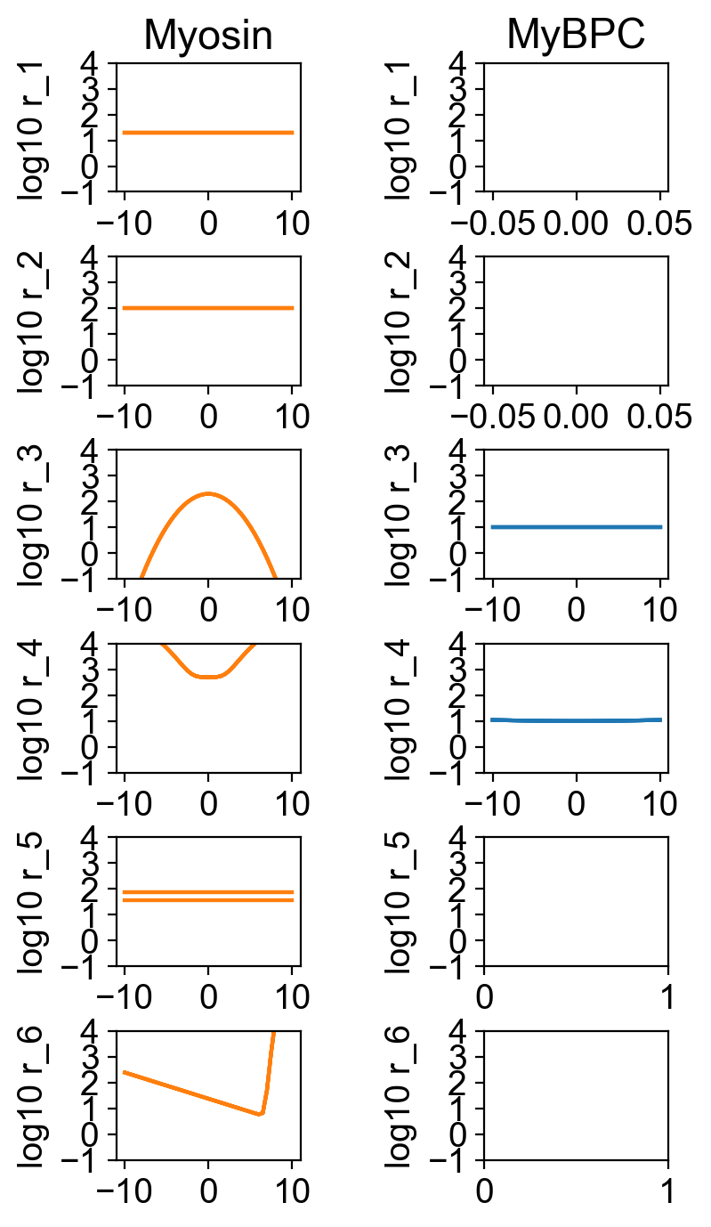
The rate constants for the different simulations are shown superposed in
How this worked
The only difference between this simulation and the single pCa curve demo is that the model section was updated to include a manipulations component.
"model":
{
    "relative_to": "this_file",
    "options_file": "sim_options.json",
    "manipulations":
    {
        "base_model": "model.json",
        "generated_folder": "../generated",
        "adjustments":
        [
            {
                "class": "thin_parameters",
                "variable": "a_k_on",
                "multipliers": [1, 0.5, 1.5, 1, 0.5],
                "output_type": "float"
            },
            {
                "variable": "m_kinetics",
                "isotype": 1,
                "state": 3,
                "transition": 2,
                "parameter_number": 1,
                "multipliers": [1, 1, 1, 0.5, 0.5],
                "output_type": "float"
            }
        ]
    }
}
The details are as follows:
"relative_to": "this_file"- defines the paths as relative to the set-up file"options_file": "sim_options.json"- the filename for the options file"base_model": "model.json"- the model to manipulate"generated_folder": "../generated"- where to store the adjusted models
            {
                "class": "thin_parameters",
                "variable": "a_k_on",
                "multipliers": [1, 0.5, 1.5, 1, 0.5],
                "output_type": "float"
            },
- Run simulations for 5 models in which
thin_parameters : a_k_onis set to 1, 0.5, 1.5, 1, and 0.5 times its value in the base model - This approach works for any model parameter that is defined as a single value within a top-level class.
            {
                "variable": "m_kinetics",
                "isotype": 1,
                "state": 3,
                "transition": 2,
                "parameter_number": 1,
                "multipliers": [1, 1, 1, 0.5, 0.5],
                "output_type": "float"
            }
- During the 5 trials adjust
parameter_number1 in the kinetics for myosinisotype1,state3,transition2 to 1, 1, 1, 0.5, 0.5 times its value in the base model - If the variable is changed to
c_kinetics, the parameters for cMyBP-C transitions will be adjusted instead.
This nomenclature is a bit more complicated but should be easier to understand when viewed in conjunction with the same section from the base model file.
"m_kinetics": [
    {
    "state": [
        {
            <snip>
        },
        {
            <snip>
        },
        {
          "number": 3,
          "type": "A",
          "extension": 0.0,
          "transition": [
            {
              "new_state": 2,
              "rate_type": "poly",
              "rate_parameters": [ 500, 10, 4]
            },
            {
                "new_state": 4,
                "rate_type": "constant",
                "rate_parameters": [ 75 ]
              }
          ]
        },
        {
            <snip>
        }
      ]
    }
  ],
This section describes the kinetics for a single myosin isoform. (There is is only one entry within the "m_kinetics": [].
The third component of the scheme describes transitions for an attached state with 0 power-stroke extension. The second transition from this state is defined by a single value (parameter_number = 1) and has a constant value corresponding to a rate of 75 s-1.
The 5 simulations are thus run with values of 75, 75, 75, 37.5, and 37.5 s-1 respectively, where 37.5 = 0.5 * 75.